![[banner]](images/banner.jpg "Cohansey River, Fairfield, New Jersey")
The Cuzick, Jonckheere–Terpstra, and Mack–Wolf Tests are used in similar circumstances as when a Kruskal–Wallis test would be used. With the difference that they each treat the independent variable as ordinal categories instead of nominal categories as in the Kruskal–Wallis test.
The Cuzick test evaluates a trend in the dependent variable across the ordered categories of the independent variable. The implementation here does not explicitly correct for ties in the dependent variable.
The Jonckheere–Terpstra test is used for a similar purpose. The implementation here does correct for ties.
The Mack–Wolf test looks for what is called an “umbrella alternative”, that is if the data have a rising trend and then a falling trend.
These tests are all nonparametric in nature.
Note that these tests make sense only if the independent variable can be considered ordered categories. And, of course, the data need to be passed to R in a way that the categories in the independent variable are ordered correctly.
Packages used in this chapter
The packages used in this chapter include:
• ggplot2
• ggbeeswarm
• rcompanion
• PMCMRplus
• DescTools
The following commands will install these packages if they are not already installed:
if(!require(ggplot2)){install.packages("ggplot2")}
if(!require(ggbeeswarm)){install.packages("ggbeeswarm")}
if(!require(rcompanion)){install.packages("rcompanion")}
if(!require(PMCMRplus)){install.packages("PMCMRplus")}
if(!require(DescTools)){install.packages("DescTools")}
Horsley soybean yield data
As an example, we’ll use the Horsley soybean data from the “Polynomial Contrasts in Models” chapter in An R Companion for the Handbook of Biological Statistics (rcompanion.org/rcompanion/h_03.html).
These data are arranged in complete randomized block design (CRBD). But the tests in this chapter will ignore the block effect. In this case, this won’t make much difference, as the block effect is not very large relative to the effect of the independent variable, Spacing.
Horsley soybean yield data
Block = rep( 1:6, each = 5)
Spacing = rep(c(18, 24, 30, 36, 42), 6)
Yield = c(33.6, 31.1, 33.0, 28.4, 31.4,
37.1, 34.5, 29.5, 29.9, 28.3,
34.1, 30.5, 29.2, 31.6, 28.9,
34.6, 32.7, 30.7, 32.3, 28.6,
35.4, 30.7, 30.7, 28.1, 29.6,
36.1, 30.3, 27.9, 26.9, 33.4)
Data = data.frame(Block = factor(Block),
Spacing = factor(Spacing),
Yield = Yield)
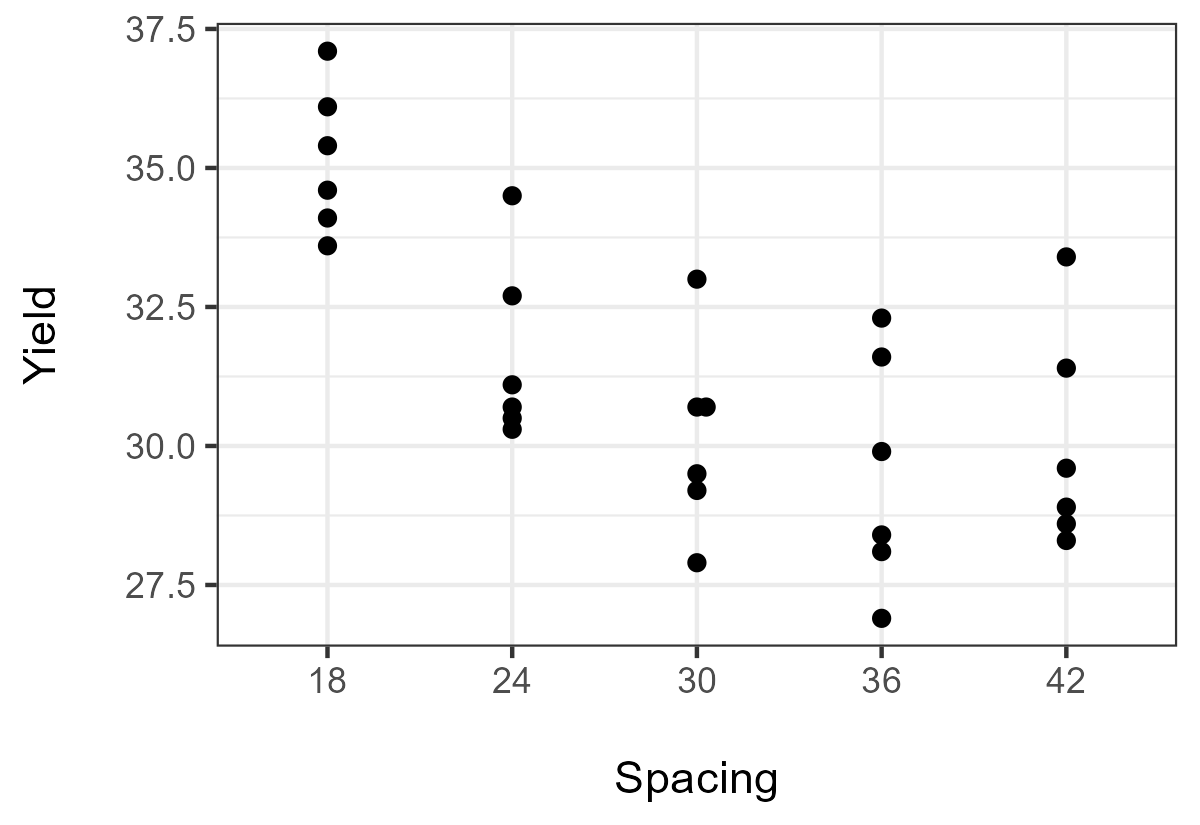
Plot
library(ggplot2)
library(ggbeeswarm)
Plot = ggplot(Data, aes(y = Yield,x = Spacing)) +
geom_beeswarm() +
theme_bw() +
xlab("\nSpacing") +
ylab("Yield\n")
ggsave(filename="Horsley.png",
plot = Plot,
width = 4,
height = 2.75,
dpi = 300,
units = "in")
Adjusting for the block effect (optional)
With this design, it’s easy to adjust the Yield values for the block effect, if we wanted to take the block effect into account.
First, we can examine the difference in the means across blocks. Here, the means of the blocks deviate from the global mean of Yield by less than 0.6, so the effect of the blocks isn’t large relative to the effect of Spacing.
mean(Data$Yield)
31.30333
library(rcompanion)
groupwiseMean(Yield ~ Block, data = Data)
Block n Mean Conf.level Trad.lower Trad.upper
1 1 5 31.5 0.95 29.0 34.0
2 2 5 31.9 0.95 27.2 36.5
3 3 5 30.9 0.95 28.2 33.5
4 4 5 31.8 0.95 29.0 34.6
5 5 5 30.9 0.95 27.5 34.3
6 6 5 30.9 0.95 26.2 35.7
library(rcompanion)
Means = groupwiseMean(Yield ~ Block, data = Data)
Data$Adjustment = Means$Mean[Data$Block] - mean(Data$Yield)
Data$Yield.Adj = Data$Yield - Data$Adjustment
library(rcompanion)
groupwiseMean(Yield.adj ~ Block, data = Data)
Block n Mean Conf.level Trad.lower Trad.upper
1 1 5 31.3 0.95 28.8 33.8
2 2 5 31.3 0.95 26.6 35.9
3 3 5 31.3 0.95 28.6 33.9
4 4 5 31.3 0.95 28.5 34.1
5 5 5 31.3 0.95 27.9 34.7
6 6 5 31.3 0.95 26.6 36.1
Cuzick test
Again, note that this implementation of Cuzick test does not correct for ties. In our Yield data, there is one value observed three times (30.7), but this shouldn’t cause a major problem. If the dependent variable were ordinal, we would want a test that corrects for ties.
The results here suggest that there is an overall trend in Yield across increasing categories of Spacing. Apparently, here, it is a decreasing trend. The negative z-value—as well as the plot of the data—suggests a negative trend.
library(PMCMRplus)
cuzickTest(Yield ~ Spacing, data=Data)
Cuzick trend test
z = -3.4462, p-value = 0.0005685
sample estimates:
CU
1160
Jonckheere–Terpstra test
Here, the Jonckheere-Terpstra test also finds a significant trend in Yield across increasing categories of Spacing. Again, the negative z-value and the plot of the data suggest a negative trend.
library(PMCMRplus)
jonckheereTest(Yield ~ Spacing, data=Data)
Jonckheere-Terpstra test
z = -3.5803, p-value = 0.0003432
sample estimates:
JT
82
library(DescTools)
JonckheereTerpstraTest(Yield ~ Spacing, data=Data)
Jonckheere-Terpstra test
JT = 82, p-value = 0.0003456
Mack–Wolf test
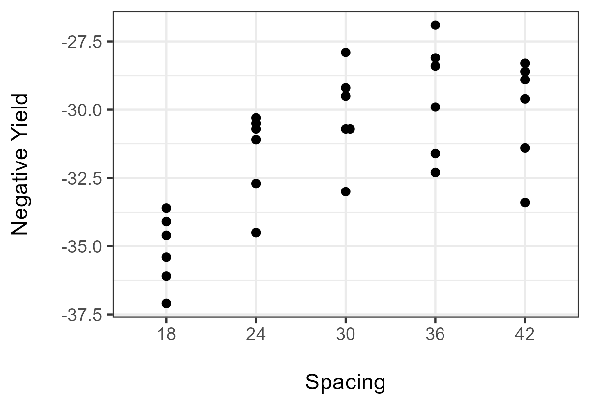
With this implementation, the Mack–Wolf test always looks for an umbrella with an increasing trend and then a decreasing trend. Because our Horsley soybean data show the opposite trend, the easiest thing is to create another variable here called YieldNegative, which is just Yield with the opposite sign.
Data$YieldNegative = 0 - Data$Yield
Plot02 = ggplot(Data, aes(y = YieldNegative,x = Spacing)) +
geom_beeswarm() +
theme_bw() +
xlab("\nSpacing") +
ylab("Negative Yield\n")
ggsave(filename="Horsley02.png",
plot = Plot02,
width = 4,
height = 2.75,
dpi = 300,
units = "in")
Mack–Wolf test with unknown peak
The Mack–Wolf test can be conducted with an unknown peak. Here, the test estimates the peak with p = 5, suggesting the change in trend direction occurs at Spacing = 42. That is, there is no umbrella effect detected, just an overall trend across all categories.
library(PMCMRplus)
mackWolfeTest(YieldNegative ~ Spacing, data=Data)
Mack-Wolfe test for umbrella alternatives with unknown peak
Ap* = 3.5419, p-value < 2.2e-16
p = 5
### Note that the p-value may change due to its
determination
### by permutation test.
Mack–Wolf test with known peak
The test can also be conducted where a hypothesized peak is identified. Here, we’ll identify a peak at p = 4, or Spacing = 36.
library(PMCMRplus)
mackWolfeTest(YieldNegative ~ Spacing, data=Data, p=4)
Mack-Wolfe test for umbrella alternatives with known peak
z = 3.2733, p-value = 0.0005316
p = 4
### Note that the p-value may change due to its
determination
### by permutation test
We could also test for a peak at p = 3.5, or Spacing between 30 and 36. The z-value for this test is slightly that for p = 4.
mackWolfeTest(YieldNegative ~ Spacing, data=Data, p=3.5)
Mack-Wolfe test for umbrella alternatives with known peak
z = 3.1651, p-value = 0.000775
p = 3.5
Neither test with a hypothesized peak has a z-value as high as that for the test with no peak value specified. Likely, we would need to see the data for Spacing = 48 to be sure that there actually is a decreasing trend in YieldNegative or spacing greater than 30 or 36.
Note on changing the direction of trend
Because implementations for each of the Cuzick test and the Jonckheere-Terpstra test here report a signed z-value and a two-sided test, these test tests will identify either an increasing trend or a decreasing trend.
We’ve already noted that the implementation of the Mack–Wolf test here necessitates an increasing then decreasing trend in the dependent variable. The test does, however, report a signed z-value. A two-sided test could be used with this z-value to detect either an umbrella response or an inverted umbrella response.
Test = mackWolfeTest(Yield ~ Spacing, data=Data, p=3.5)
Test$statistic
z
-2.087649
2*pnorm(q=abs(-2.087649), lower.tail=FALSE)
0.03682951
### p-value for a two-sided test
My understanding is that the Ap* statistic reported by the test without a specified peak value can be used as an estimate of the z-value.
Test = mackWolfeTest(Yield ~ Spacing, data=Data)
Test$statistic
Ap*
3.541939
2*pnorm(q=abs(3.541939), lower.tail=FALSE)
0.0003971973
### p-value for a two-sided test
References
Horsley, R.D. No date. Orthogonal Polynomial Contrasts Individual Df Comparisons: Equally Spaced Treatments. North Dakota State University. rcompanion.org/documents/Polycnst.pdf.