R Handbook: Measures of Association for Nominal Variables

There are several statistics that can be used to gauge the strength of the association between two nominal variables. They are used as measures of effect size for tests of association for nominal variables.

The statistics phi and Cramér’s V are commonly used. Cramér’s V varies from 0 to 1, with a 1 indicting a perfect association. phi varies from –1 to 1, with –1 and 1 indicating perfect associations. phi is available only for 2 x 2 tables.

Cohen’s w is similar to Cramér’s V in use, but it’s upper value is not limited to 1.

The odds ratio is appropriate for some contingency tables. It is useful when the table describes a bivariate response among groups. For example, disease or no disease among males and females. Or, pass or fail among locations.

Cohen’s h is used to compare the difference in two proportions. It can be used in 2 x 2 contingency tables in cases where it makes sense to compare the proportions in rows or columns. It can also be used in cases where proportions are known but the actual counts are not. A value of 0 indicates no difference in proportions, and the difference between proportions of 0.00 and 1.00 results in a value of ± pi (c. 3.14).

Goodman and Kruskal’s lambda statistic is also used to gauge the strength of the association between two nominal variables. It is formulated so that one dimension on the table is considered the independent variable, and one is considered the dependent variable, so that the independent variable is used to predict the dependent variable. It varies from 0 to 1.

Another measure of association is Tschuprow's T. It is similar to Cramér’s V, and they are equivalent for square tables (one with an equal number of rows and columns).

Appropriate data

• Two nominal variables with two or more levels each. Usually expressed as a contingency table.

• Experimental units aren’t paired.

• For phi, the table is 2 x 2 only.

• For odds ratio, one variable is bivariate. That is, it has two levels.

Hypotheses

• There are no hypotheses tested directly with these statistics.

Other notes and alternative tests

• Freeman’s theta and epsilon squared are used for tables with one ordinal variable and one nominal variable.

• For tables with two ordinal variables, Kendall’s Tau-b, Goodman and Kruskal's gamma, and Somers’ D are used.

Interpretation of statistics

The interpretation of measures of association is always relative to the discipline, the specific data, and the aims of the analyst. Sometimes guidelines are given for “small”, “medium”, and “large” effects—for example from Cohen (1988) for behavioral sciences—but it is important to remember that these are still relative to the discipline and type of data. A smaller effect size may be considered “large” in psychology or behavioral science, but may be considered quite small in a physical science such as chemistry. The specific conditions of the study are important as well. For example, one would expect the difference in knowledge between a group completely ignorant of a subject and one educated in the subject to be large, but the difference between two groups educated in the same subject with different methods might be small.

The interpretation for odds ratio presented here was derived from that for Cohen’s h, for 2 x 2 tables. Note that the cutoffs for interpretation for odds ratio shown here are different from those given in the Tests for Paired Nominal Data chapter, and are different than those from other internet sources.

	Small	Medium	Large
Cohen’s w	0.10 – < 0.30	0.30 – < 0.50	≥ 0.50
*phi*	0.10 – < 0.30	0.30 – < 0.50	≥ 0.50
Cohen’s h	0.20 – < 0.50	0.50 – < 0.80	≥ 0.80
Cramér’s V, k = 2^*	0.10 – < 0.30	0.30 – < 0.50	≥ 0.50
Cramér’s V, k = 3^*	0.07 – < 0.20	0.20 – < 0.35	≥ 0.35
Cramér’s V, k = 4^*	0.06 – < 0.17	0.17 – < 0.29	≥ 0.29
Odds ratio	1.53 – < 3.00	3.00 – < 6.52	≥ 6.52

________________________________
Adapted from Cohen (1988).

^* k is the minimum number of categories in either rows or columns.

Packages used in this chapter

The packages used in this chapter include:

• rcompanion

• vcd

• psych

• DescTools

• epitools

The following commands will install these packages if they are not already installed:

if(!require(rcompanion)){install.packages("rcompanion")}
if(!require(vcd)){install.packages("vcd")}
if(!require(psych)){install.packages("psych")}
if(!require(DescTools)){install.packages("DescTools")}
if(!require(epitools)){install.packages("epitools")}

Examples for measures of association for nominal variables

Cramér’s V

Input =("
County               Pass   Fail
Bloom                21      5
Cobblestone           6     11
Dougal                7      8
Heimlich             27      5
")

Matrix = as.matrix(read.table(textConnection(Input),
                   header=TRUE,
                   row.names=1))

Matrix

library(rcompanion)

cramerV(Matrix,
        digits=4)

Cramer V
0.4387

library(vcd)

assocstats(Matrix)

Phi-Coefficient : NA
Cramer's V : 0.439

library(DescTools)

CramerV(Matrix,
conf.level=0.95)

Cramer V lwr.ci upr.ci
0.4386881 0.1944364 0.6239856

phi

Input =("
Sex      Pass Fail
Male     49   64
Female   44   24
")

Matrix.2 = as.matrix(read.table(textConnection(Input),
                     header=TRUE,
                     row.names=1))

Matrix.2

library(psych)

phi(Matrix.2,
    digits = 4)

[1] -0.2068

library(DescTools)

Phi(Matrix.2)

[1] 0.206808

### It appears that DescTools always produces a positive value.

library(rcompanion)

cramerV(Matrix.2)

Cramer V

0.2068

### Note that Cramer’s V is the same as the absolute value
### of phi for 2 x 2 tables.

Odds ratio

The oddsratio function in the epitools package calculates the odds ratio for a contingency table of two responses, given in the columns, and treatments or groups given in rows. By default, the function assumes that the top row is the control group. The function can calculate the odds ratio a few different ways. If the option method=“wald” is used, the result for the first example would be the same as the odds of Female failing (24/44) divided by the odds of Male failing (64/49), or 0.418. The calculation by the default median unbiased estimation is slightly different. For tables larger than 2 x 2, the top row is used as the control for each other row.

Input =("
Sex      Pass Fail
Male     49   64
Female   44   24
")

Matrix.2 = as.matrix(read.table(textConnection(Input),
                     header=TRUE,
                     row.names=1))

Matrix.2

library(epitools)

oddsratio(Matrix.2)$measure

odds ratio with 95% C.I. estimate     lower     upper
                  Male   1.000000        NA        NA
                  Female 0.420623 0.2229345 0.7791587

odds ratio with 95% C.I. estimate    lower     upper
             Bloom       1.0000000       NA        NA
             Cobblestone 7.1542726 1.846641 32.389543
             Dougal      4.5405648 1.123581 20.551625
             Heimlich    0.7813714 0.186609 3.265344

Cohen’s w

Cohen w
0.4387

   ### Note that because the smallest dimension in the table is 2,
       the value of Cohen’s w is the same as that for
       Cramer’s V.

Cohen’s h

Input =("
Sex      Pass Fail
Male     49   64
Female   44   24
")

Matrix.2 = as.matrix(read.table(textConnection(Input),
                     header=TRUE,
                     row.names=1))

Matrix.2

library(rcompanion)

cohenH(Matrix.2,
       observation = "row",
       digits = 3)

   Group Proportion
1   Male      0.434
2 Female      0.647

Cohen's h
    0.432

Goodman Kruskal lambda

[1] 0.2068966

### County predicts Pass/Fail

Tschuprow's T

[1] 0.3333309

Optional analysis: using effect size statistics when counts are not known

One property of effect size statistics is that they are not affected by sample size. This allows some to be used when proportions are known for a contingency table, but actual counts are not known.

As an example, we could analyze the proportions of votes for the Democratic candidate in 2016 and 2018 in Pennsylvania’s 18^th Congressional District. The 2016 data are for the presidential race where Hilary Clinton was the Democratic candidate. The 2018 data are for the House of Representatives election where Conor Lamb was the Democratic candidate.

Note that the effect sizes here are considered “small” by Cohen’s guidelines, but notable for American politics at the national level.

Input =("
     Democrat Not.Democrat
2016    0.380        0.620
2018    0.498        0.502
")

Penn18 = as.matrix(read.table(textConnection(Input),
                   header=TRUE,
                   row.names=1))

Penn18

   Democrat Not.Democrat
2016    0.380        0.620
2018    0.498        0.502

library(rcompanion)

cohenH(Penn18,
observation = "row",
digits = 3)

Group Proportion
1 2016      0.380
2 2018      0.498

Cohen's h
   0.238

library(psych)

phi(Penn18,
digits = 3)

[1] -0.119

library(rcompanion)

cramerV(Penn18,
digits=3)

Cramer V

0.119

Optional analysis: Cohen’s h and prop.test for paired data when subject matching isn’t known

In the chapter on Tests for Paired Nominal Data, there is an example measuring rain barrel adoption before and after a class.

In this example, the identity of subjects was matched before and after, and the table could be analyzed with McNemar’s test or a similar test, and the effect size could be determined with Cohen’s g.

Before       After.yes   After.no
Before.yes     9         5
Before.no     17         15

However, if the subjects identities were not recorded in a manner that allowed for this matching, we could still measure the difference in proportions with Cohen’s h and with prop.test.

Input =("
Time       Yes   No
Before     14   32
After     26   20
")

Unmatched = as.matrix(read.table(textConnection(Input),
                      header=TRUE,
                      row.names=1))

Unmatched

library(rcompanion)

cohenH(Unmatched,
       observation = "row",
       digits = 3)

   Group Proportion
1 Before      0.304
2 After      0.565

Cohen's h
    0.533

Yes = c(14, 26)
Trials = c(14+32, 26+20)
prop.test(Yes, Trials)

2-sample test for equality of proportions with continuity correction

data: Yes out of Trials
X-squared = 5.3519, df = 1, p-value = 0.0207
alternative hypothesis: two.sided
95 percent confidence interval:
-0.47806470 -0.04367443
sample estimates:
prop 1 prop 2
0.3043478 0.5652174

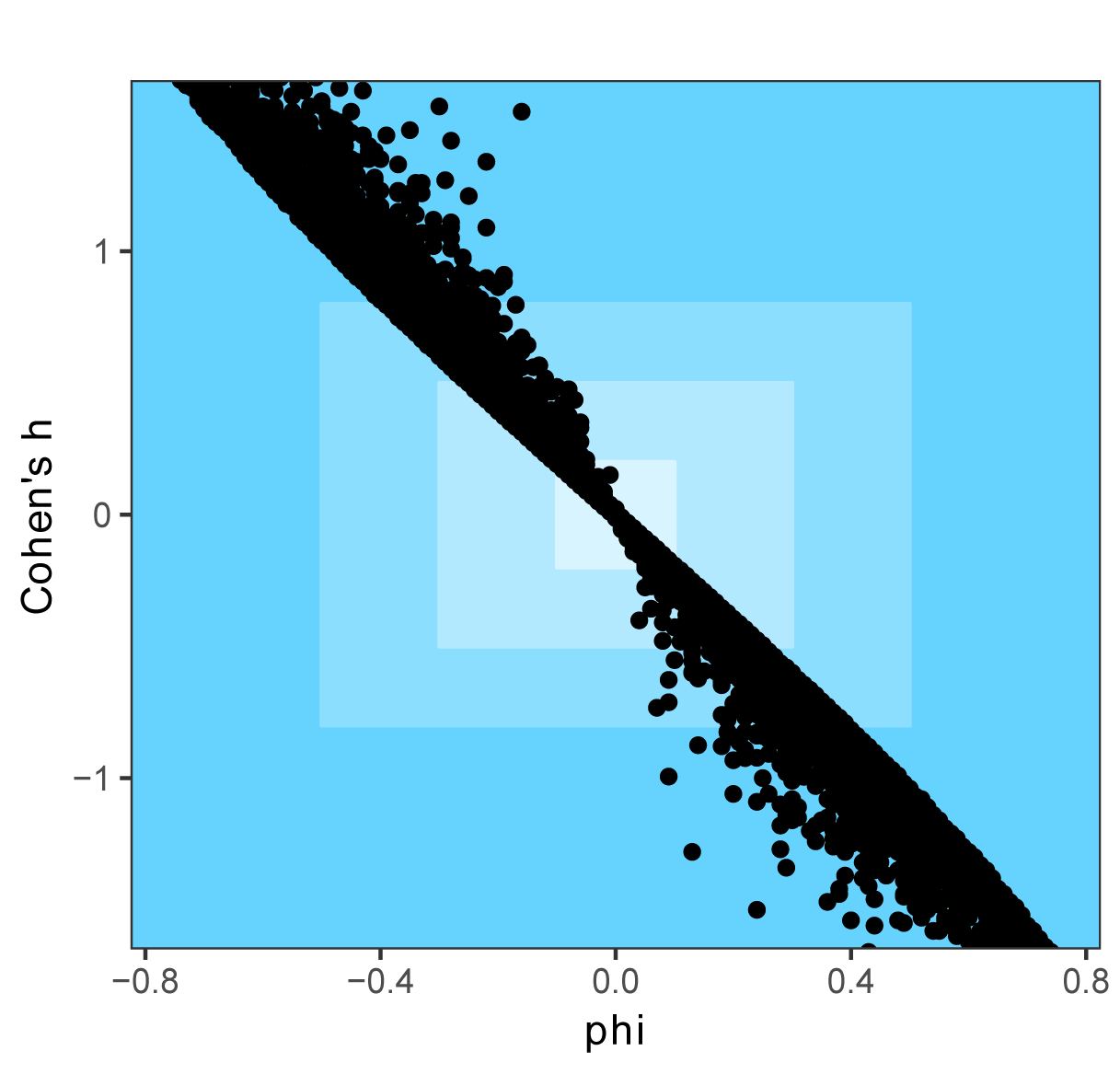
Optional: Comparing phi and Cohen’s h for a 2 x 2 table

For a 2 x 2 table, Cohen’s h and phi do not follow a strictly monotonic relationship. Both statistics equal zero when there is no relationship, and Cohen’s h approaches pi as phi approaches –1. (As calculated here, the statistics have a negative relationship.) But there is variability in their values in between these endpoints for some simulated data.

In the second figure below, the colors indicate Cohen’s interpretation of less-than-small, small, medium, and large as the blue becomes darker. Note that the interpretations across the two statistics may vary for the same data, as is evidenced by the fact that the plotted values do not go through the corner of the rectangle delineating the medium and large interpretations. For example, for a phi of approximately –0.40 (medium), Cohen’s h are likely to range from 0.82 to 1.17, which would be interpreted as a large effect.

Optional analysis: changing the order of the table

Note that if we change the order of the rows in the table, the results for Cramér’s V, Cohen’s w, and lambda (with direction=column) do not change. This is because these statistics treat the variables as nominal and not ordinal.

Input =("
County               Pass   Fail
Heimlich             27      5
Bloom                21      5
Dougal                7      8
Cobblestone           6    11
")

Matrix.3 = as.matrix(read.table(textConnection(Input),
                     header=TRUE,
                     row.names=1))

Matrix.3

### Cramer’s V

library(rcompanion)

cramerV(Matrix.3,
digits=4)

Cramer V
0.4387

### Cohen’s w

cohenW(Matrix.3)

Cohen w
0.4387

### Goodman Kruskal lambda

library(DescTools)

Lambda(Matrix.3,
direction="column")

### Treat County as independent variable

[1] 0.2068966

Optional analysis: comparing statistics

The following examples may give some sense of the difference between Cramér’s V, and lambda.

Input =("
X    Y1   Y2
X1   10    0
X2    0   10
")

Matrix.x = as.matrix(read.table(textConnection(Input),
                   header=TRUE,
                   row.names=1))

library(rcompanion)

cramerV(Matrix.x)

Cramer V
1

library(rcompanion)

cohenW(Matrix.x)

Cohen w

library(DescTools)

Lambda(Matrix.x,
direction="column")

[1] 1

Input =("
X    Y1   Y2
X1   10    0
X2   10   10
")

Matrix.y = as.matrix(read.table(textConnection(Input),
                   header=TRUE,
                   row.names=1))

library(rcompanion)

cramerV(Matrix.y)

Cramer V
0.5

library(rcompanion)

cohenW(Matrix.y)

Cohen w
0.5

library(DescTools)

Lambda(Matrix.y,

direction="column")

[1] 0

### X predicts Y.

Input =("
X    Y1   Y2
X1   10    0
X2   10   10
X3   10   20
X4   10 30
")

Matrix.z = as.matrix(read.table(textConnection(Input),
                   header=TRUE,
                   row.names=1))

library(rcompanion)

cramerV(Matrix.z)

Cramer V
0.4488

library(rcompanion)

cohenW(Matrix.z)

Cohen w
0.4488

library(DescTools)

Lambda(Matrix.z,
direction="column")

[1] 0.25

### X predicts Y.

References

Cohen, J. 1988. Statistical Power Analysis for the Behavioral Sciences, 2nd Edition. Routledge.

Summary and Analysis of Extension Program Evaluation in R

Measures of Association for Nominal Variables