![[banner]](images/banner.jpg "Cohansey River, Fairfield, New Jersey")
Transforming data is one step in addressing data that do not fit model assumptions, and is also used to coerce different variables to have similar distributions. Before transforming data, see the “Steps to handle violations of assumption” section in the Assessing Model Assumptions chapter.
Transforming data
Most parametric tests require that residuals be normally distributed and that the residuals be homoscedastic.
One approach when residuals fail to meet these conditions is to transform one or more variables to better follow a normal distribution. Often, just the dependent variable in a model will need to be transformed. However, in complex models and multiple regression, it is sometimes helpful to transform both dependent and independent variables that deviate greatly from a normal distribution.
There is nothing illicit in transforming variables, but you must be careful about how the results from analyses with transformed variables are reported. For example, looking at the turbidity of water across three locations, you might report, “Locations showed a significant difference in log-transformed turbidity.” To present means or other summary statistics, you might present the mean of transformed values, or back transform means to their original units.
Some measurements in nature are naturally normally distributed. Other measurements are naturally log-normally distributed. These include some natural pollutants in water: There may be many low values with fewer high values and even fewer very high values.
For right-skewed data—tail is on the right, positive skew—, common transformations include square root, cube root, and log.
For left-skewed data—tail is on the left, negative skew—, common transformations include square root (constant – x), cube root (constant – x), and log (constant – x).
Because log (0) is undefined—as is the log of any negative number—, when using a log transformation, a constant should be added to all values to make them all positive before transformation. It is also sometimes helpful to add a constant when using other transformations.
Another approach is to use a general power transformation, such as Tukey’s Ladder of Powers or a Box–Cox transformation. These determine a lambda value, which is used as the power coefficient to transform values. X.new = X ^ lambda for Tukey, and X.new = (X ^ lambda – 1) / lambda for Box–Cox.
The function transformTukey in the rcompanion package finds the lambda which makes a single vector of values—that is, one variable—as normally distributed as possible with a simple power transformation.
The Box–Cox procedure is included in the MASS package with the function boxcox. It uses a log-likelihood procedure to find the lambda to use to transform the dependent variable for a linear model (such as an ANOVA or linear regression). It can also be used on a single vector.
Packages used in this chapter
The packages used in this chapter include:
• car
• MASS
• rcompanion
The following commands will install these packages if they are not already installed:
if(!require(psych)){install.packages("car")}
if(!require(MASS)){install.packages("MASS")}
if(!require(rcompanion)){install.packages("rcompanion")}
Example of transforming skewed data
This example uses hypothetical data of river water turbidity. Turbidity is a measure of how cloudy water is due to suspended material in the water. Water quality parameters such as this are often naturally log-normally distributed: values are often low, but are occasionally high or very high.
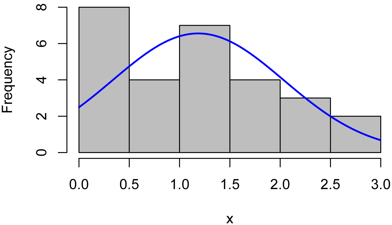
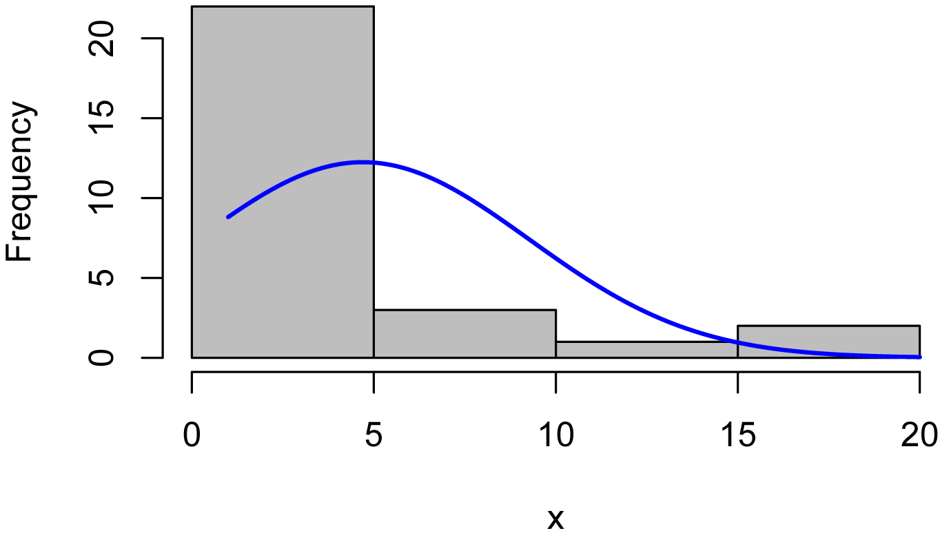
The first plot is a histogram of the Turbidity values, with a normal curve superimposed. Looking at the gray bars, this data is skewed strongly to the right (positive skew), and looks more or less log-normal. The gray bars deviate noticeably from the red normal curve.
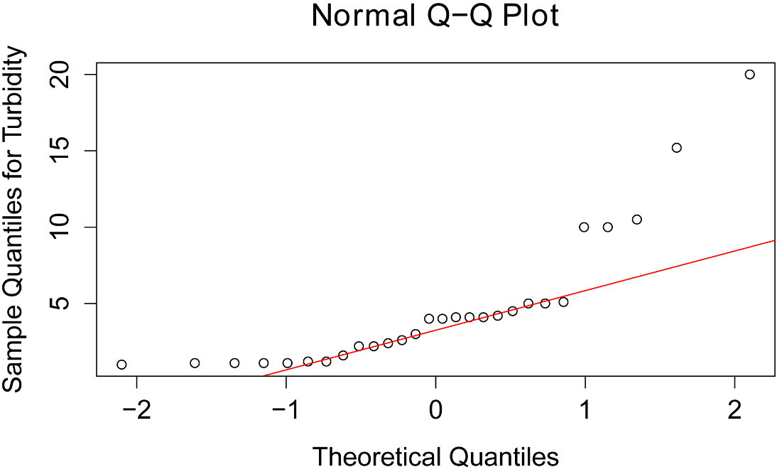
The second plot is a normal quantile plot (normal Q–Q plot). If the data were normally distributed, the points would follow the red line fairly closely.
Turbidity = c(1.0, 1.2, 1.1, 1.1, 2.4, 2.2, 2.6, 4.1, 5.0, 10.0,
4.0, 4.1, 4.2, 4.1, 5.1, 4.5, 5.0, 15.2, 10.0, 20.0, 1.1, 1.1, 1.2, 1.6, 2.2,
3.0, 4.0, 10.5)
library(rcompanion)
plotNormalHistogram(Turbidity)

qqnorm(Turbidity,
ylab="Sample Quantiles for Turbidity")
qqline(Turbidity,
col="red")
Square root transformation
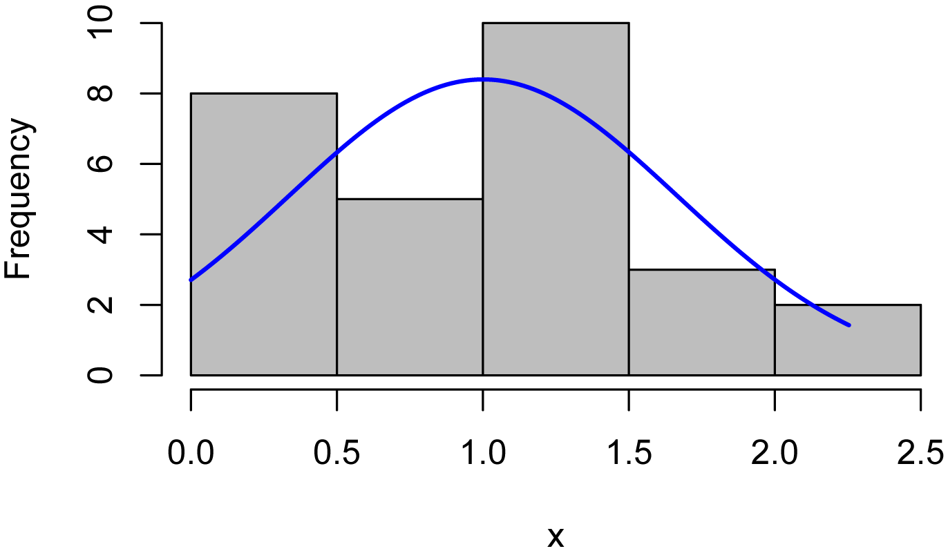
Since the data is right-skewed, we will apply common transformations for right-skewed data: square root, cube root, and log. The square root transformation improves the distribution of the data somewhat.
T_sqrt = sqrt(Turbidity)
library(rcompanion)
plotNormalHistogram(T_sqrt)

Cube root transformation
The cube root transformation is stronger than the square root transformation.
T_cub = sign(Turbidity) * abs(Turbidity)^(1/3) # Avoid complex numbers
#
for some cube roots
library(rcompanion)
plotNormalHistogram(T_cub)

Log transformation
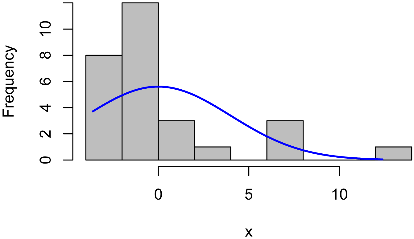
The log transformation is a relatively strong transformation. Because certain measurements in nature are naturally log-normal, it is often a successful transformation for certain data sets. While the transformed data here does not follow a normal distribution very well, it is probably about as close as we can get with these particular data.
T_log = log(Turbidity)
library(rcompanion)
plotNormalHistogram(T_log)
Tukey’s Ladder of Powers transformation
The approach of Tukey’s Ladder of Powers uses a power transformation on a data set. For example, raising data to a 0.5 power is equivalent to applying a square root transformation; raising data to a 0.33 power is equivalent to applying a cube root transformation.
Here, I use the transformTukey function, which performs iterative Shapiro–Wilk tests, and finds the lambda value that maximizes the W statistic from those tests. In essence, this finds the power transformation that makes the data fit the normal distribution as closely as possible with this type of transformation.
Left skewed values should be adjusted with (constant – value), to convert the skew to right skewed, and perhaps making all values positive. In some cases of right skewed data, it may be beneficial to add a constant to make all data values positive before transformation. For large values, it may be helpful to scale values to a more reasonable range.
In this example, the resultant lambda of –0.1 is slightly stronger than a log transformation, since a log transformation corresponds to a lambda of 0.
library(rcompanion)
T_tuk =
transformTukey(Turbidity,
plotit=FALSE)
lambda W Shapiro.p.value
397 -0.1 0.935 0.08248
if (lambda > 0){TRANS = x ^ lambda}
if (lambda == 0){TRANS = log(x)}
if (lambda < 0){TRANS = -1 * x ^ lambda}
library(rcompanion)
plotNormalHistogram(T_tuk)

Example of Tukey-transformed data in ANOVA
For an example of how transforming data can improve the distribution of the residuals of a parametric analysis, we will use the same turbidity values, but assign them to three different locations.
Transforming the turbidity values to be more normally distributed, both improves the distribution of the residuals of the analysis and makes a more powerful test, lowering the p-value.
Input =("
Location Turbidity
a 1.0
a 1.2
a 1.1
a 1.1
a 2.4
a 2.2
a 2.6
a 4.1
a 5.0
a 10.0
b 4.0
b 4.1
b 4.2
b 4.1
b 5.1
b 4.5
b 5.0
b 15.2
b 10.0
b 20.0
c 1.1
c 1.1
c 1.2
c 1.6
c 2.2
c 3.0
c 4.0
c 10.5
")
Data = read.table(textConnection(Input),header=TRUE)
Attempt ANOVA on un-transformed data
Here, even though the analysis of variance results in a significant p-value (p = 0.03), the residuals deviate from the normal distribution enough to make the analysis invalid. The plot of the residuals vs. the fitted values shows that the residuals are somewhat heteroscedastic, though not terribly so.
boxplot(Turbidity ~ Location,
data = Data,
ylab="Turbidity",
xlab="Location")
model = lm(Turbidity ~ Location,
data=Data)
library(car)
Anova(model, type="II")
Anova Table (Type II tests)
Sum Sq Df F value Pr(>F)
Location 132.63 2 3.8651 0.03447 *
Residuals 428.95 25
x = (residuals(model))
library(rcompanion)
plotNormalHistogram(x)

qqnorm(residuals(model),
ylab="Sample Quantiles for residuals")
qqline(residuals(model),
col="red")

plot(fitted(model),
residuals(model))

Transform data
library(rcompanion)
Data$Turbidity_tuk =
transformTukey(Data$Turbidity,
plotit=FALSE)
lambda W Shapiro.p.value
397 -0.1 0.935 0.08248
if (lambda > 0){TRANS = x ^ lambda}
if (lambda == 0){TRANS = log(x)}
if (lambda < 0){TRANS = -1 * x ^ lambda}
ANOVA with Tukey-transformed data
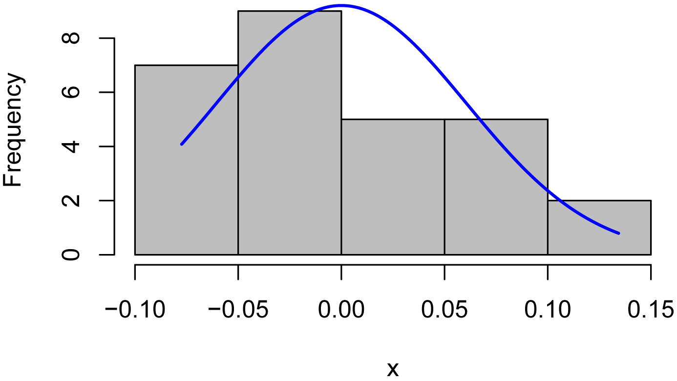
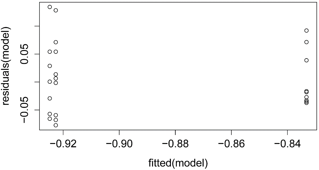
After transformation, the residuals from the ANOVA are closer to a normal distribution—although not perfectly—, making the F-test more appropriate. In addition, the test is more powerful as indicated by the lower p-value (p = 0.005) than with the untransformed data. The plot of the residuals vs. the fitted values shows that the residuals are about as heteroscedastic as they were with the untransformed data.
boxplot(Turbidity_tuk ~ Location,
data = Data,
ylab="Tukey-transformed Turbidity",
xlab="Location")

model = lm(Turbidity_tuk ~ Location,
data=Data)
library(car)
Anova(model, type="II")
Anova Table (Type II tests)
Sum Sq Df F value Pr(>F)
Location 0.052506 2 6.6018 0.004988 **
Residuals 0.099416 25
x = residuals(model)
library(rcompanion)
plotNormalHistogram(x)
qqnorm(residuals(model),
ylab="Sample Quantiles for residuals")
qqline(residuals(model),
col="red")

plot(fitted(model),
residuals(model))
Box–Cox transformation
The Box–Cox procedure is similar in concept to the Tukey Ladder of Power procedure described above. However, instead of transforming a single variable, it maximizes a log-likelihood statistic for a linear model (such as ANOVA or linear regression). It will also work on a single variable using a formula of x ~ 1.
The Box–Cox procedure is available with the boxcox function in the MASS package. However, a few steps are needed to extract the lambda value and transform the data set.
This example uses the same turbidity data.
Turbidity = c(1.0, 1.2, 1.1, 1.1, 2.4, 2.2, 2.6, 4.1, 5.0, 10.0, 4.0, 4.1, 4.2,
4.1, 5.1, 4.5, 5.0, 15.2, 10.0, 20.0, 1.1, 1.1, 1.2, 1.6, 2.2, 3.0, 4.0, 10.5)
library(rcompanion)
plotNormalHistogram(Turbidity)
qqnorm(Turbidity,
ylab="Sample Quantiles for Turbidity")
qqline(Turbidity,
col="red")
Box–Cox transformation for a single variable
library(MASS)
Box = boxcox(Turbidity ~ 1, # Transform
Turbidity as a single vector
lambda = seq(-6,6,0.1) # Try
values -6 to 6 by 0.1
)
Cox = data.frame(Box$x, Box$y) # Create
a data frame with the results
Cox2 = Cox[with(Cox, order(-Cox$Box.y)),] # Order the
new data frame by decreasing y
Cox2[1,] # Display
the lambda with the greatest
# log likelihood
Box.x Box.y
59 -0.2 -41.35829
lambda = Cox2[1, "Box.x"] # Extract that lambda
T_box = (Turbidity ^ lambda - 1)/lambda # Transform
the original data
library(rcompanion)
plotNormalHistogram(T_box)
Example of Box–Cox transformation for ANOVA model
Input =("
Location Turbidity
a 1.0
a 1.2
a 1.1
a 1.1
a 2.4
a 2.2
a 2.6
a 4.1
a 5.0
a 10.0
b 4.0
b 4.1
b 4.2
b 4.1
b 5.1
b 4.5
b 5.0
b 15.2
b 10.0
b 20.0
c 1.1
c 1.1
c 1.2
c 1.6
c 2.2
c 3.0
c 4.0
c 10.5
")
Data = read.table(textConnection(Input),header=TRUE)
Attempt ANOVA on un-transformed data
model = lm(Turbidity ~ Location,
data=Data)
library(car)
Anova(model, type="II")
Anova Table (Type II tests)
Sum Sq Df F value Pr(>F)
Location 132.63 2 3.8651 0.03447 *
Residuals 428.95 25
x = residuals(model)
library(rcompanion)
plotNormalHistogram(x)
qqnorm(residuals(model),
ylab="Sample Quantiles for residuals")
qqline(residuals(model),
col="red")
plot(fitted(model),
residuals(model))
Transform data
library(MASS)
Box = boxcox(Turbidity ~ Location,
data = Data,
lambda = seq(-6,6,0.1)
)
Cox = data.frame(Box$x, Box$y)
Cox2 = Cox[with(Cox, order(-Cox$Box.y)),]
Cox2[1,]
lambda = Cox2[1, "Box.x"]
Data$Turbidity_box = (Data$Turbidity ^ lambda - 1)/lambda
boxplot(Turbidity_box ~ Location,
data = Data,
ylab="Box–Cox-transformed Turbidity",
xlab="Location")

Perform ANOVA and check residuals
model = lm(Turbidity_box ~ Location,
data=Data)
library(car)
Anova(model, type="II")
Anova Table (Type II tests)
Sum Sq Df F value Pr(>F)
Location 0.16657 2 6.6929 0.0047 **
Residuals 0.31110 25
x = residuals(model)
library(rcompanion)
plotNormalHistogram(x)

qqnorm(residuals(model),
ylab="Sample Quantiles for residuals")
qqline(residuals(model),
col="red")

plot(fitted(model),
residuals(model))

Conclusions
Both the Tukey’s Ladder of Powers principle as implemented by the transformTukey function and the Box–Cox procedure were successful at transforming a single variable to follow a more normal distribution. They were also both successful at improving the distribution of residuals from a simple ANOVA.
The Box–Cox procedure has the advantage of dealing with the dependent variable of a linear model, while the transformTukey function works only for a single variable without considering other variables. Because of this, the Box–Cox procedure may be advantageous when a relatively simple model is considered. In cases where there are complex models or multiple regression, it may be helpful to transform both dependent and independent variables independently.