![[banner]](images/banner.jpg "Cohansey River, Fairfield, New Jersey")
When an experimental design takes measurements on the same experimental unit over time, the analysis of the data must take into account the probability that measurements for a given experimental unit will be correlated in some way. For example, if we were measuring calorie intake for students, we would expect that if one student had a higher intake at Time 1, that that student would have a higher intake others at Time 2, and so on.
In previous chapters, our approach to deal with non-independent observations was to treat Student as a blocking variable or as a random (blocking) variable.
The approach in this chapter is to include an autocorrelation structure in the model using the nmle package.
Packages used in this chapter
The packages used in this chapter include:
• psych
• nlme
• car
• multcompView
• lsmeans
• ggplot2
• rcompanion
The following commands will install these packages if they are not already installed:
if(!require(psych)){install.packages("psych")}
if(!require(nlme)){install.packages("nlme")}
if(!require(car)){install.packages("car")}
if(!require(multcompView)){install.packages("multcompView")}
if(!require(lsmeans)){install.packages("lsmeans")}
if(!require(ggplot2)){install.packages("ggplot2")}
if(!require(rcompanion)){install.packages("rcompanion")}
Repeated measures ANOVA example
In this example, students were asked to document their daily caloric intake once a month for six months. Students were divided into three groups with each receiving instruction in nutrition education using one of three curricula.
There are different ways we might approach this problem. If we simply wanted to see if one curriculum was better at decreasing caloric intake in students, we might do a simple analysis of variance on the difference between each student’s final and initial intake.
In the approach here we will use a repeated measures analysis with all the measurements, treating Student as a random variable to take into account native differences among students, and including an autocorrelation structure.
Data = read.table(header=TRUE, stringsAsFactors=TRUE, text="
Instruction Student Month Calories.per.day
'Curriculum A' a 1 2000
'Curriculum A' a 2 1978
'Curriculum A' a 3 1962
'Curriculum A' a 4 1873
'Curriculum A' a 5 1782
'Curriculum A' a 6 1737
'Curriculum A' b 1 1900
'Curriculum A' b 2 1826
'Curriculum A' b 3 1782
'Curriculum A' b 4 1718
'Curriculum A' b 5 1639
'Curriculum A' b 6 1644
'Curriculum A' c 1 2100
'Curriculum A' c 2 2067
'Curriculum A' c 3 2065
'Curriculum A' c 4 2015
'Curriculum A' c 5 1994
'Curriculum A' c 6 1919
'Curriculum A' d 1 2000
'Curriculum A' d 2 1981
'Curriculum A' d 3 1987
'Curriculum A' d 4 2016
'Curriculum A' d 5 2010
'Curriculum A' d 6 1946
'Curriculum B' e 1 2100
'Curriculum B' e 2 2004
'Curriculum B' e 3 2027
'Curriculum B' e 4 2109
'Curriculum B' e 5 2197
'Curriculum B' e 6 2294
'Curriculum B' f 1 2000
'Curriculum B' f 2 2011
'Curriculum B' f 3 2089
'Curriculum B' f 4 2124
'Curriculum B' f 5 2199
'Curriculum B' f 6 2234
'Curriculum B' g 1 2000
'Curriculum B' g 2 2074
'Curriculum B' g 3 2141
'Curriculum B' g 4 2199
'Curriculum B' g 5 2265
'Curriculum B' g 6 2254
'Curriculum B' h 1 2000
'Curriculum B' h 2 1970
'Curriculum B' h 3 1951
'Curriculum B' h 4 1981
'Curriculum B' h 5 1987
'Curriculum B' h 6 1969
'Curriculum C' i 1 1950
'Curriculum C' i 2 2007
'Curriculum C' i 3 1978
'Curriculum C' i 4 1965
'Curriculum C' i 5 1984
'Curriculum C' i 6 2020
'Curriculum C' j 1 2000
'Curriculum C' j 2 2029
'Curriculum C' j 3 2033
'Curriculum C' j 4 2050
'Curriculum C' j 5 2001
'Curriculum C' j 6 1988
'Curriculum C' k 1 2000
'Curriculum C' k 2 1976
'Curriculum C' k 3 2025
'Curriculum C' k 4 2047
'Curriculum C' k 5 2033
'Curriculum C' k 6 1984
'Curriculum C' l 1 2000
'Curriculum C' l 2 2020
'Curriculum C' l 3 2009
'Curriculum C' l 4 2017
'Curriculum C' l 5 1989
'Curriculum C' l 6 2020
")
### Order factors by the order in data frame
### Otherwise, R will alphabetize them
Data$Instruction = factor(Data$Instruction,
levels=unique(Data$Instruction))
### Check the data frame
library(psych)
headTail(Data)
str(Data)
summary(Data)
Define model and conduct analysis of deviance
This example will use a mixed effects model to describe the repeated measures analysis, using the lme function in the nlme package. Student is treated as a random variable in the model.
The autocorrelation structure is described with the correlation statement. In this case, corAR1 is used to indicate a temporal autocorrelation structure of order one, often abbreviated as AR(1). This statement takes the form:
correlation = Structure(form = ~ time | subjvar)
where:
• Structure is the autocorrelation structure. Options are listed in library(nlme); ?corClasses
• time is the variable indicating time. In this case, Month. For the corAR1 structure, the time variable must be an integer variable.
• subjvar indicates the variable for experimental units, in this case Student. Autocorrelation is modeled within levels of the subjvar, and not between them.
For the corAR1 structure, a value for the first order correlation can be specified. In this case, the value of 0.429 is found using the ACF function in the “Optional analysis: determining autocorrelation in residuals” section below.
Autocorrelation structures can be chosen by either of two methods. The first is to choose a structure based on theoretical expectations of how the data should be correlated. The second is to try various autocorrelation structures and compare the resulting models with a criterion like AIC, AICc, or BIC to choose the structure that best models the data.
Optional technical note:
In this case, it isn’t necessary to use a mixed effects model. That is, it’s not necessary to include Student as a random variable. A similar analysis could be conducted by using the gls function in the nlme package, and including the correlation option, but excluding the random option, as follows in black.
library(nlme)
model = gls(Calories.per.day ~ Instruction + Month + Instruction*Month,
correlation = corAR1(form = ~ Month | Student,
value = 0.8990),
data=Data,
method="REML")
library(car)
Anova(model)
Code for analysis
library(nlme)
model = lme(Calories.per.day ~ Instruction + Month + Instruction*Month,
random = ~1|Student,
correlation = corAR1(form = ~ Month | Student,
value = 0.4287),
data=Data,
method="REML")
library(car)
Anova(model)
Analysis of Deviance Table (Type II tests)
Response: Calories.per.day
Chisq Df Pr(>Chisq)
Instruction 10.4221 2 0.005456 **
Month 0.0198 1 0.888045
Instruction:Month 38.6045 2 4.141e-09 ***
Test the random effects in the model
The random effects in the model can be tested by comparing the model to a model fitted with just the fixed effects and excluding the random effects. Because there are not random effects in this second model, the gls function in the nlme package is used to fit this model.
model.fixed = gls(Calories.per.day ~ Instruction + Month + Instruction*Month,
data=Data,
method="REML")
anova(model,
model.fixed)
Model df AIC BIC logLik Test L.Ratio p-value
model 1 9 716.9693 736.6762 -349.4847
model.fixed 2 7 813.6213 828.9489 -399.8106 1 vs 2 100.652 <.0001
p-value and pseudo R-squared for model
The nagelkerke function can be used to calculate a p-value and pseudo R-squared value for the model.
One approach is to define the null model as one with no fixed effects except for an intercept, indicated with a 1 on the right side of the ~. And to also include the random effects, in this case 1|Student.
library(rcompanion)
model.null =
lme(Calories.per.day ~ 1,
random = ~1|Student,
data = Data)
nagelkerke(model,
model.null)
$Pseudo.R.squared.for.model.vs.null
Pseudo.R.squared
McFadden 0.123969
Cox and Snell (ML) 0.768652
Nagelkerke (Cragg and Uhler) 0.768658
$Likelihood.ratio.test
Df.diff LogLik.diff Chisq p.value
-6 -52.698 105.4 1.8733e-20
Another approach to determining the p-value and pseudo R-squared for an lme model is to compare the model to a null model with only an intercept and neither the fixed nor the random effects. To accomplish this, the null model has to be specified with the gls function.
library(rcompanion)
model.null.2
= gls(Calories.per.day ~ 1,
data = Data)
nagelkerke(model,
model.null.2)
$Pseudo.R.squared.for.model.vs.null
Pseudo.R.squared
McFadden 0.168971
Cox and Snell (ML) 0.877943
Nagelkerke (Cragg and Uhler) 0.877946
$Likelihood.ratio.test
Df.diff LogLik.diff Chisq p.value
-7 -75.717 151.43 2.0282e-29
Post-hoc analysis
The lsmeans package is able to handle lme objects. For further details, see ?lsmeans::models. For a review of mean separation tests and least square means, see the chapters What are Least Square Means?; the chapter Least Square Means for Multiple Comparisons; and the “Post-hoc analysis: mean separation tests” section in the One-way ANOVA chapter.
Because Month is an integer variable, not a factor variable, it is listed in the lsmeans cld table as its average only.
library(multcompView)
library(lsmeans)
marginal = lsmeans(model,
~ Instruction:Month)
cld(marginal,
alpha = 0.05,
Letters = letters, ### Use lower-case
letters for .group
adjust = "tukey") ### Tukey-adjusted
comparisons
Instruction Month lsmean SE df lower.CL upper.CL .group
Curriculum A 3.5 1907.601 42.83711 11 1787.206 2027.996 a
Curriculum C 3.5 1997.429 42.83711 9 1872.222 2122.637 ab
Curriculum B 3.5 2102.965 42.83711 9 1977.758 2228.172 b
Confidence level used: 0.95
Conf-level adjustment: sidak method for 3 estimates
P value adjustment: tukey method for comparing a family of 3 estimates
significance level used: alpha = 0.05.05
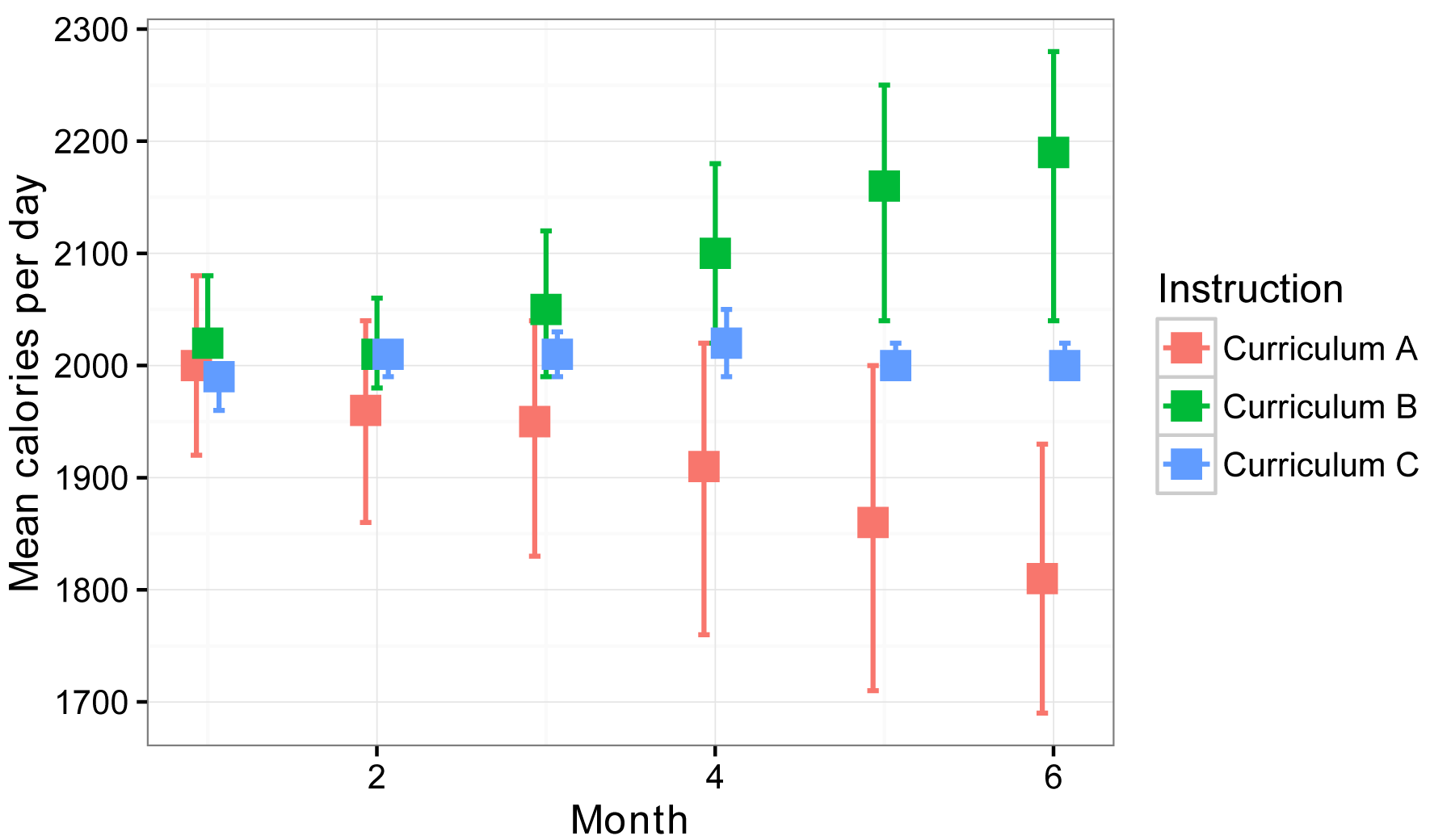
Interaction plot
For this plot, we will use the groupwiseMean function to calculate the natural mean of each Instruction x Month combination, along with the confidence interval of each mean with the percentile method.
library(rcompanion)
Sum = groupwiseMean(Calories.per.day ~ Instruction + Month,
data = Data,
conf = 0.95,
digits = 3,
traditional = FALSE,
percentile = TRUE)
Sum
Instruction Month n Mean Conf.level Percentile.lower Percentile.upper
1 Curriculum A 1 4 2000 0.95 1920 2080
2 Curriculum A 2 4 1960 0.95 1860 2040
3 Curriculum A 3 4 1950 0.95 1830 2040
4 Curriculum A 4 4 1910 0.95 1760 2020
5 Curriculum A 5 4 1860 0.95 1710 2000
6 Curriculum A 6 4 1810 0.95 1690 1930
7 Curriculum B 1 4 2020 0.95 2000 2080
8 Curriculum B 2 4 2010 0.95 1980 2060
9 Curriculum B 3 4 2050 0.95 1990 2120
10 Curriculum B 4 4 2100 0.95 2020 2180
11 Curriculum B 5 4 2160 0.95 2040 2250
12 Curriculum B 6 4 2190 0.95 2040 2280
13 Curriculum C 1 4 1990 0.95 1960 2000
14 Curriculum C 2 4 2010 0.95 1990 2020
15 Curriculum C 3 4 2010 0.95 1990 2030
16 Curriculum C 4 4 2020 0.95 1990 2050
17 Curriculum C 5 4 2000 0.95 1990 2020
18 Curriculum C 6 4 2000 0.95 1990 2020
library(ggplot2)
pd = position_dodge(.2)
ggplot(Sum, aes(x = Month,
y = Mean,
color = Instruction)) +
geom_errorbar(aes(ymin=Percentile.lower,
ymax=Percentile.upper),
width=.2, size=0.7, position=pd) +
geom_point(shape=15, size=4, position=pd) +
theme_bw() +
theme(axis.title = element_text(face = "bold")) +
ylab("Mean calories per day")
Histogram of residuals
Residuals from a mixed model fit with nlme should be normally distributed. Plotting residuals vs. fitted values, to check for homoscedasticity and independence, is probably also advisable.
x = residuals(model)
library(rcompanion)
plotNormalHistogram(x)

plot(fitted(model),
residuals(model))

Optional analysis: determining autocorrelation in residuals
The ACF function in the nlme package will indicate the autocorrelation for lags in the time variable. Note that for a gls model, the form of the autocorrelation structure can be specified. For an lme model, the function uses the innermost group level and assumes equally spaced intervals.
library(nlme)
model.a = gls(Calories.per.day ~ Instruction + Month + Instruction*Month,
data=Data)
ACF(model.a,
form = ~ Month | Student)
lag ACF
1 0 1.0000000
2 1 0.8989822
3 2 0.7462712
4 3 0.6249217
5 4 0.5365430
6 5 0.4564673
library(nlme)
model.b = lme(Calories.per.day ~ Instruction + Month + Instruction*Month,
random = ~1|Student,
data=Data)
ACF(model.b)
lag ACF
1 0 1.0000000
2 1 0.4286522
3 2 -0.1750233
4 3 -0.6283754
5 4 -0.8651088
6 5 -0.6957774
Optional discussion on specifying formulae for repeated measures analysis
Specifying random effects in models
The general schema for specifying random effects in R is:
Formula.for.random.effects | Unit.for.which.these.apply
So that, in the nlme package:
• random = ~ 1 | subject
Indicates that each subject will have its own intercept
• random = ~ rep | subject
Indicates that each subject will have its own intercept and its own slope for rep
• random = ~ 1 | rep/subject
Indicates that each subject-within-rep unit will have its own intercept
Indicating time and subject variables
A simple repeated analysis statement in proc mixed in SAS could be specified with:
repeated date / subject = id type = AR(1)
A similar specification in with the gls function in nlme package in R would be:
correlation = corAR1(form = ~ date | id)
Likewise, a simple mixed effects repeated analysis statement in proc mixed in SAS could be specified with:
random id
repeated date / subject = id type = AR(1)
A similar specification in with the lme function in nlme package in R would be:
random = ~1 | id,
correlation = corAR1(form = ~ date | id)
Specifying nested effects
In repeated measures analysis, it is common to used nested effects. For example, if our subject variable is treatment within block,
In SAS:
treatment(block)
is equivalent to
block block*treatment
In R:
block/treatment
is equivalent to
block + block:treatment