Summary and Analysis of Extension Program Evaluation in R

Salvatore S. Mangiafico

Two-way ANOVA

A two-way anova can investigate the main effects of each of two independent factor variables, as well as the effect of the interaction of these variables.

 

For an overview of the concepts in multi-way analysis of variance, review the chapter Factorial ANOVA: Main Effects, Interaction Effects, and Interaction Plots.

 

For a review of mean separation tests and least square means, see the chapters What are Least Square Means?; the chapter Least Square Means for Multiple Comparisons; and the “Post-hoc analysis:  mean separation tests” section in the One-way ANOVA chapter.

 

Appropriate data

•  Two-way data.  That is, one dependent variable measured across two independent factor variables

•  Dependent variable is interval/ratio, and is continuous

•  Independent variables are a factor with two or more levels.  That is, two or more groups for each independent variable

•  In the general linear model approach, residuals are normally distributed

•  In the general linear model approach, groups have the same variance.  That is, homoscedasticity

•  Observations among groups are independent.  That is, not paired or repeated measures data

•  Moderate deviation from normally-distributed residuals is permissible

 

Hypotheses

•  Null hypothesis 1:  The means of the dependent variable for each group in the first independent variable are equal

•  Alternative hypothesis 1 (two-sided): The means of the dependent variable for each group in the first independent variable are not equal

•  Similar hypotheses are considered for the other independent variable

•  Similar hypotheses are considered for the interaction effect

 

Interpretation

•  Reporting significant results for the effect of one independent variable as “Significant differences were found among means for groups.” is acceptable.  Alternatively, “A significant effect for independent variable on dependent variable was found.”

•  Reporting significant results for the interaction effect as “A significant effect for the interaction of independent variable 1 and independent variable 2 on dependent variable was found.” Is acceptable.

•  Reporting significant results for mean separation post-hoc tests as “Mean of variable Y for group A was different than that for group B.” is acceptable.

 

Packages used in this chapter

 

The packages used in this chapter include:

•  psych

•  FSA

•  car

•  multcompView

•  lsmeans

•  Rmisc

•  ggplot2

•  rcompanion

 

The following commands will install these packages if they are not already installed:

if(!require(psych)){install.packages("psych")}
if(!require(FSA)){install.packages("FSA")}
if(!require(car)){install.packages("car")}
if(!require(multcompView)){install.packages("multcompView")}
if(!require(lsmeans)){install.packages("lsmeans")}
if(!require(Rmisc)){install.packages("Rmisc")}
if(!require(ggplot2)){install.packages("ggplot2")}
if(!require(rcompanion)){install.packages("rcompanion")}

Two-way ANOVA example

 

This example will revisit the sodium intake data set with Brendon Small and the other instructors.  This time, though, they want to test not only the different nutrition education programs (indicated by Instructor), but also four supplements to the program, each of which they have used with some students. 

Input = ("
Instructor        Supplement  Sodium
'Brendon Small'   A           1200
'Brendon Small'   A           1400
'Brendon Small'   A           1350
'Brendon Small'   A            950
'Brendon Small'   A           1400
'Brendon Small'   B           1150
'Brendon Small'   B           1300
'Brendon Small'   B           1325
'Brendon Small'   B           1425
'Brendon Small'   B           1500
'Brendon Small'   C           1250
'Brendon Small'   C           1150
'Brendon Small'   C            950
'Brendon Small'   C           1150
'Brendon Small'   C           1600
'Brendon Small'   D           1300
'Brendon Small'   D           1050
'Brendon Small'   D           1300
'Brendon Small'   D           1700
'Brendon Small'   D           1300
'Coach McGuirk'   A           1100
'Coach McGuirk'   A           1200
'Coach McGuirk'   A           1250
'Coach McGuirk'   A           1050
'Coach McGuirk'   A           1200
'Coach McGuirk'   B           1250
'Coach McGuirk'   B           1350
'Coach McGuirk'   B           1350
'Coach McGuirk'   B           1325
'Coach McGuirk'   B           1525
'Coach McGuirk'   C           1225
'Coach McGuirk'   C           1125
'Coach McGuirk'   C           1000
'Coach McGuirk'   C           1125
'Coach McGuirk'   C           1400
'Coach McGuirk'   D           1200
'Coach McGuirk'   D           1150
'Coach McGuirk'   D           1400
'Coach McGuirk'   D           1500
'Coach McGuirk'   D           1200
'Melissa Robins'  A            900
'Melissa Robins'  A           1100
'Melissa Robins'  A           1150
'Melissa Robins'  A            950
'Melissa Robins'  A           1100
'Melissa Robins'  B           1150
'Melissa Robins'  B           1250
'Melissa Robins'  B           1250
'Melissa Robins'  B           1225
'Melissa Robins'  B           1325
'Melissa Robins'  C           1125
'Melissa Robins'  C           1025
'Melissa Robins'  C            950
'Melissa Robins'  C            925
'Melissa Robins'  C           1200
'Melissa Robins'  D           1100
'Melissa Robins'  D            950
'Melissa Robins'  D           1300
'Melissa Robins'  D           1400
'Melissa Robins'  D           1100
")

Data = read.table(textConnection(Input),header=TRUE)

###  Order factors by the order in data frame
###  Otherwise, R will alphabetize them

Data$Instructor = factor(Data$Instructor,
                         levels=unique(Data$Instructor))

Data$Supplement       = factor(Data$Supplement,
                         levels=unique(Data$Supplement))


###  Check the data frame

library(psych)

headTail(Data)

str(Data)

summary(Data)


### Remove unnecessary objects

rm(Input)

Use Summarize to check if cell sizes are balanced

We can use the n or nvalid columns in the Summarize output to check if cell sizes are balanced.  That is, if each combination of treatments have the same number of observations.

library(FSA)

Summarize(Sodium ~ Supplement + Instructor,
          data=Data,
          digits=3)

   Supplement     Instructor n mean      sd  min   Q1 median   Q3  max
1           A  Brendon Small 5 1260 191.703  950 1200   1350 1400 1400
2           B  Brendon Small 5 1340 132.994 1150 1300   1325 1425 1500
3           C  Brendon Small 5 1220 238.747  950 1150   1150 1250 1600
4           D  Brendon Small 5 1330 233.452 1050 1300   1300 1300 1700
5           A  Coach McGuirk 5 1160  82.158 1050 1100   1200 1200 1250
6           B  Coach McGuirk 5 1360 100.933 1250 1325   1350 1350 1525
7           C  Coach McGuirk 5 1175 148.955 1000 1125   1125 1225 1400
8           D  Coach McGuirk 5 1290 151.658 1150 1200   1200 1400 1500
9           A Melissa Robins 5 1040 108.397  900  950   1100 1100 1150
10          B Melissa Robins 5 1240  62.750 1150 1225   1250 1250 1325
11          C Melissa Robins 5 1045 116.458  925  950   1025 1125 1200
12          D Melissa Robins 5 1170 178.885  950 1100   1100 1300 1400

Define linear model

Note that the interaction of Instruction and Supplement is indicated in the model definition by Instructor:Supplement.

model = lm(Sodium ~ Instructor + Supplement + Instructor:Supplement,
           data = Data)


summary(model)   ### Will show overall p-value and r-square

Multiple R-squared:  0.3491,  Adjusted R-squared:    0.2

F-statistic: 2.341 on 11 and 48 DF,  p-value: 0.02121

Conduct analysis of variance

library(car)

Anova(model,
      type = "II")   ### Type II sum of squares

Anova Table (Type II tests)

Response: Sodium
                       Sum Sq Df F value   Pr(>F)  
Instructor             290146  2  6.0173 0.004658 **
Supplement             306125  3  4.2324 0.009841 **
Instructor:Supplement   24438  6  0.1689 0.983880  
Residuals             1157250 48                   

Histogram of residuals

x = residuals(model)


library(rcompanion)

plotNormalHistogram(x)

plot(fitted(model),
     residuals(model))

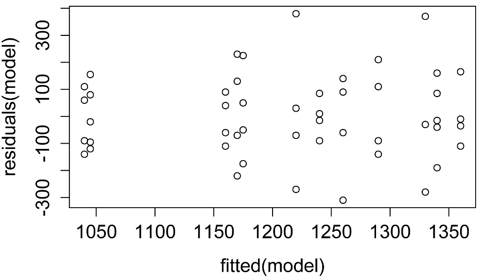
plot(model)   ### Additional model checking plots

Post-hoc analysis:  mean separation tests

For an explanation of using least square means for multiple comparisons, see the section “Post-hoc analysis:  mean separation tests” in the One-way ANOVA chapter.

 

LS means for main effects

library(multcompView)

library(lsmeans)

marginal = lsmeans(model,
                   ~ Instructor)

pairs(marginal,
      adjust="tukey")

contrast                        estimate      SE df t.ratio p.value
 Brendon Small - Coach McGuirk     41.25 49.1013 48   0.840  0.6802
 Brendon Small - Melissa Robins   163.75 49.1013 48   3.335  0.0046
 Coach McGuirk - Melissa Robins   122.50 49.1013 48   2.495  0.0418

Results are averaged over the levels of: Supplement
P value adjustment: tukey method for comparing a family of 3 estimates

CLD = cld(marginal,
          alpha   = 0.05,
          Letters = letters,         ###  Use lowercase letters for .group
          adjust  = "tukey")         ###  Tukey-adjusted comparisons

CLD

Instructor      lsmean       SE df lower.CL upper.CL .group
 Melissa Robins 1123.75 34.71986 48 1053.941 1193.559  a   
 Coach McGuirk  1246.25 34.71986 48 1176.441 1316.059   b  
 Brendon Small  1287.50 34.71986 48 1217.691 1357.309   b  

Results are averaged over the levels of: Supplement
Confidence level used: 0.95
P value adjustment: tukey method for comparing a family of 3 estimates
significance level used: alpha = 0.05

library(multcompView)

library(lsmeans)

marginal = lsmeans(model,
                   ~ Supplement)

pairs(marginal,
      adjust="tukey")

contrast    estimate      SE df t.ratio p.value
 A - B    -160.000000 56.6973 48  -2.822  0.0338
 A - C       6.666667 56.6973 48   0.118  0.9994
 A - D    -110.000000 56.6973 48  -1.940  0.2253
 B - C     166.666667 56.6973 48   2.940  0.0251
 B - D      50.000000 56.6973 48   0.882  0.8142
 C - D    -116.666667 56.6973 48  -2.058  0.1818

Results are averaged over the levels of: Instructor
P value adjustment: tukey method for comparing a family of 4 estimates

CLD = cld(marginal,
          alpha   = 0.05,
          Letters = letters,      ###  Use lowercase letters for .group
          adjust  = "tukey")      ###  Tukey-adjusted comparisons

CLD

Supplement   lsmean       SE df lower.CL upper.CL .group
 C          1146.667 40.09104 48 1066.058 1227.275  a   
 A          1153.333 40.09104 48 1072.725 1233.942  a   
 D          1263.333 40.09104 48 1182.725 1343.942  ab  
 B          1313.333 40.09104 48 1232.725 1393.942   b  

Results are averaged over the levels of: Instructor
Confidence level used: 0.95
P value adjustment: tukey method for comparing a family of 4 estimates
significance level used: alpha = 0.05

Plot of means and confidence intervals for main effects

Because the interaction term was not significant, we would probably want to present means for the main effects only.  Some authors would suggest re-doing the analysis without the interaction included.

 

For different data, the nudge_y parameter will need to be adjusted manually.

library(multcompView)

library(lsmeans)

marginal = lsmeans(model,
                   ~ Instructor)


CLD = cld(marginal,
          alpha   = 0.05,
          Letters = letters,         ###  Use lowercase letters for .group
          adjust  = "tukey")         ###  Tukey-adjusted comparisons


### Order the levels for printing

CLD$Instructor = factor(CLD$Instructor,
                        levels=c("Brendon Small",

                                 "Coach McGuirk",

                                 "Melissa Robins"))

###  Remove spaces in .group 

CLD$.group=gsub(" ", "", CLD$.group)


### Plot

library(ggplot2)

ggplot(CLD,
       aes(x     = Instructor,
           y     = lsmean,
           label = .group)) +

    geom_point(shape  = 15,
               size   = 4) +

    geom_errorbar(aes(ymin  =  lower.CL,
                      ymax  =  upper.CL),
                      width =  0.2,
                      size  =  0.7) +

    theme_bw() +
    theme(axis.title   = element_text(face = "bold"),
          axis.text    = element_text(face = "bold"),
          plot.caption = element_text(hjust = 0)) +

    ylab("Least square mean\nsodium intake (mg / day)") +

  geom_text(nudge_x = c(0, 0, 0),
            nudge_y = c(120, 120, 120),
            color   = "black")

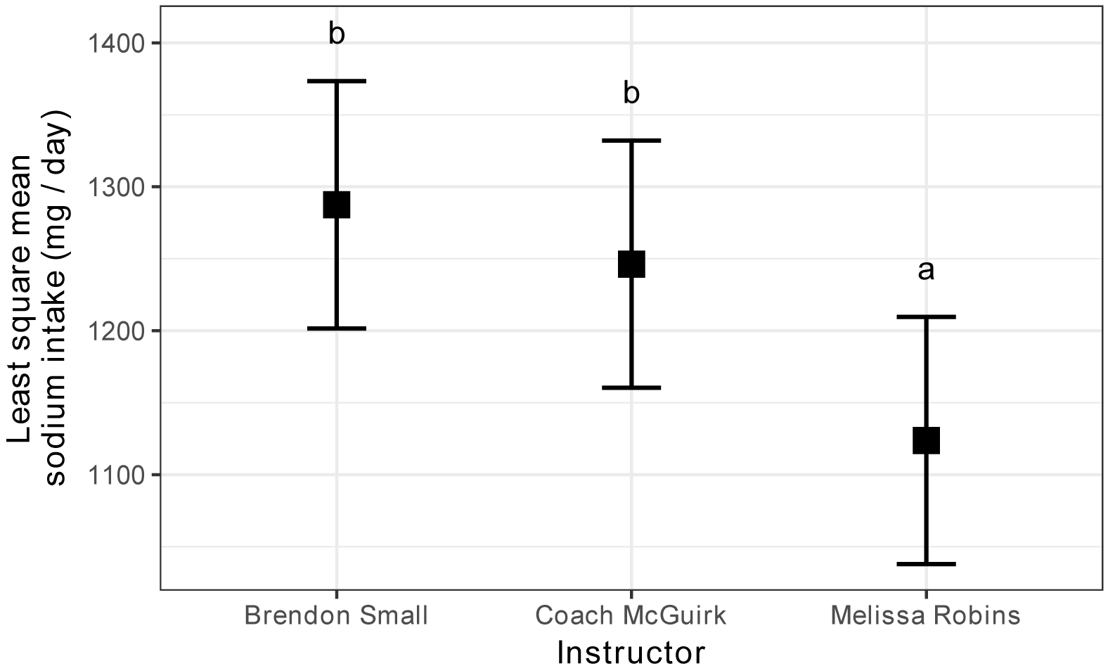
Least square mean daily sodium intake for students in each of three classes with four different supplemental programs.  Error bars indicate confidence intervals for the least square means.  Groups sharing the same letter are not significantly different (alpha = 0.05, Tukey-adjusted).

library(multcompView)

library(lsmeans)

marginal = lsmeans(model,
                   ~ Supplement)


CLD = cld(marginal,
          alpha   = 0.05,
          Letters = letters,         ###  Use lowercase letters for .group
          adjust  = "tukey")         ###  Tukey-adjusted comparisons


### Order the levels for printing

CLD$Supplement = factor(CLD$Supplement,
                        levels=c("A", "B", "C", "D"))


###  Remove spaces in .group 

CLD$.group=gsub(" ", "", CLD$.group)


### Plot

library(ggplot2)

ggplot(CLD,
       aes(x     = Supplement,
           y     = lsmean,
           label = .group)) +

    geom_point(shape  = 15,
               size   = 4) +

    geom_errorbar(aes(ymin  =  lower.CL,
                      ymax  =  upper.CL),
                      width =  0.2,
                      size  =  0.7) +

    theme_bw() +
    theme(axis.title   = element_text(face = "bold"),
          axis.text    = element_text(face = "bold"),
          plot.caption = element_text(hjust = 0)) +

    ylab("Least square mean\nsodium intake (mg / day)") +

  geom_text(nudge_x = c(0, 0, 0, 0),
            nudge_y = c(140, 140, 140, 140),
            color   = "black")

Least square mean daily sodium intake for students in each of three classes with four different supplemental programs.  Error bars indicate confidence intervals for the least square means.  Groups sharing the same letter are not significantly different (alpha = 0.05, Tukey-adjusted).

Plot of LS means and confidence intervals for interaction

If the interaction effect were significant, it would make sense to present an interaction plot of the means for both main effects together on one plot.  We can indicate mean separations with letters on the plot.

 

For different data, the nudge_y parameter will need to be adjusted manually.

library(multcompView)

library(lsmeans)

marginal = lsmeans(model,
                   ~ Instructor + Supplement)


CLD = cld(marginal,
          alpha   = 0.05,
          Letters = letters,         ###  Use lowercase letters for .group
          adjust  = "tukey")         ###  Tukey-adjusted comparisons


### Order the levels for printing

CLD$Instructor = factor(CLD$Instructor,
                        levels=c("Brendon Small",

                                 "Coach McGuirk",

                                 "Melissa Robins"))

CLD$Supplement = factor(CLD$Supplement,
                        levels=c("A", "B", "C", "D"))


###  Remove spaces in .group 

CLD$.group=gsub(" ", "", CLD$.group)


CLD


### Plot

library(ggplot2)

pd = position_dodge(0.6)    ### How much to jitter the points on the plot

ggplot(CLD,
       aes(x     = Instructor,
           y     = lsmean,
           color = Supplement,
           label = .group)) +

    geom_point(shape  = 15,
               size   = 4,
             position = pd) +

    geom_errorbar(aes(ymin  =  lower.CL,
                      ymax  =  upper.CL),
                      width =  0.2,
                      size  =  0.7,
                      position = pd) +

    theme_bw() +
    theme(axis.title   = element_text(face = "bold"),
          axis.text    = element_text(face = "bold"),
          plot.caption = element_text(hjust = 0)) +

  ylab("Least square mean\nsodium intake (mg / day)") +
 
  geom_text(nudge_x = c(-0.22, 0.08, -0.22, 0.22,
                         0.08, 0.08, -0.08, -0.22,
                         0.22, 0.22, -0.08, -0.08),
            nudge_y = rep(270, 12),
            color   = "black") +
 
  scale_color_manual(values = c("steelblue", "steelblue2",
                                "springgreen4", "springgreen3"))

Least square mean daily sodium intake for students in each of three classes with four different supplemental programs.  Error bars indicate confidence intervals for the least square means.  Groups sharing the same letter are not significantly different (alpha = 0.05, Tukey-adjusted).

Exercises T

 

1. Considering Brendon, Melissa, and McGuirk’s data with for instructional programs and supplements,

a.  Is the experimental design balanced?

 

b.  Does Instructor have a significant effect on sodium intake?

c.  Does Supplement have a significant effect on sodium intake?

 

d.  Does the interaction of Instructor and Supplement have a significant effect on sodium intake?

 

e.  Are the residuals from the analysis reasonably normal and homoscedastic?

f.  Which instructors had classes with significantly different mean sodium intake from which others?

g.  Does this result correspond to what you would have thought from looking at the plot of the LS means and confidence intervals?

 

h.  How would you summarize the effect of the supplements?

2.  As part of a professional skills program, a 4-H club tests its members for typing proficiency.  Dr. Katz, and Laura, and Ben want to compare their students’ mean typing speed between their classes, as well as for the software they used to teach typing.

Instructor                             Software  Words.per.minute
'Dr. Katz Professional Therapist'      A         35
'Dr. Katz Professional Therapist'      A         50
'Dr. Katz Professional Therapist'      A         55
'Dr. Katz Professional Therapist'      A         60
'Dr. Katz Professional Therapist'      B         65
'Dr. Katz Professional Therapist'      B         60
'Dr. Katz Professional Therapist'      B         70
'Dr. Katz Professional Therapist'      B         55
'Dr. Katz Professional Therapist'      C         45
'Dr. Katz Professional Therapist'      C         55
'Dr. Katz Professional Therapist'      C         60
'Dr. Katz Professional Therapist'      C         45
'Laura the Receptionist'               A         55
'Laura the Receptionist'               A         60
'Laura the Receptionist'               A         75
'Laura the Receptionist'               A         65
'Laura the Receptionist'               B         60
'Laura the Receptionist'               B         70
'Laura the Receptionist'               B         75
'Laura the Receptionist'               B         70
'Laura the Receptionist'               C         65
'Laura the Receptionist'               C         72
'Laura the Receptionist'               C         73
'Laura the Receptionist'               C         65
'Ben Katz'                             A         55
'Ben Katz'                             A         55
'Ben Katz'                             A         70
'Ben Katz'                             A         55
'Ben Katz'                             B         65
'Ben Katz'                             B         60
'Ben Katz'                             B         70
'Ben Katz'                             B         60
'Ben Katz'                             C         60
'Ben Katz'                             C         62
'Ben Katz'                             C         63
'Ben Katz'                             C         65

For each of the following, answer the question, and show the output from the analyses you used to answer the question.

 

a.  What was the LS mean typing speed for each instructor’s class?

b.  Does Instructor have a significant effect on typing speed?

c.  Does Software have a significant effect on typing speed?

d.  Are the residuals reasonably normal and homoscedastic?

e.  Which instructors had classes with significantly different mean typing speed from which others?

 

f.  How do you summarize the results of the effect of Software.

g.  What is your summary of the analysis and practical conclusions?

©2016 by Salvatore S. Mangiafico.
Rutgers Cooperative Extension, New Brunswick, NJ.
Updated: 2025.

Non-commercial reproduction of this content, with attribution, is permitted.
For-profit reproduction without permission is prohibited.

If you use the code or information in this site in a published work, please cite it as a source.  Also, if you are an instructor and use this book in your course, please let me know.   My contact information is on the About the Author of this Book page.

Citation

Mangiafico, S.S. 2016. Summary and Analysis of Extension Program Evaluation in R, version 1.23.0, revised 2025. rcompanion.org/handbook/. (Pdf version: rcompanion.org/documents/RHandbookProgramEvaluation.pdf.)