![[banner]](images/banner.jpg "Cohansey River, Fairfield, New Jersey")
Initial comments
Traditionally when students first learn about the analysis of experiments, there is a strong focus on hypothesis testing and making decisions based on p-values. Hypothesis testing is important for determining if there are statistically significant effects. However, readers of this book should not place undo emphasis on p-values. Instead, they should realize that p-values are affected by sample size, and that a low p-value does not necessarily suggest a large effect or a practically meaningful effect. Summary statistics, plots, effect size statistics, and practical considerations should be used. The goal is to determine: a) statistical significance, b) effect size, c) practical importance. These are all different concepts, and they will be explored below.
Statistical inference
Most of what we’ve covered in this book so far is about producing descriptive statistics: calculating means and medians, plotting data in various ways, and producing confidence intervals. The bulk of the rest of this book will cover statistical inference: using statistical tests to draw some conclusion about the data. We’ve already done this a little bit in earlier chapters by using confidence intervals to conclude if means are different or not among groups.
As Dr. Nic mentions in her article in the “References and further reading” section, this is the part where people sometimes get stumped. It is natural for most of us to use summary statistics or plots, but jumping to statistical inference needs a little change in perspective. The idea of using some statistical test to answer a question isn’t a difficult concept, but some of the following discussion gets a little theoretical. The video from the Statistics Learning Center in the “References and further reading” section does a good job of explaining the basis of statistical inference.
One important thing to gain from this chapter is an understanding of how to use the p-value, alpha, and decision rule to test the null hypothesis. But once you are comfortable with that, you will want to return to this chapter to have a better understanding of the theory behind this process.
Another important thing is to understand the limitations of relying on p-values, and why it is important to assess the size of effects and weigh practical considerations.
Packages used in this chapter
The packages used in this chapter include:
• lsr
The following commands will install these packages if they are not already installed:
if(!require(lsr)){install.packages("lsr")}
Hypothesis testing
The null and alternative hypotheses
The statistical tests in this book rely on testing a null hypothesis, which has a specific formulation for each test. The null hypothesis always describes the case where e.g. two groups are not different or there is no correlation between two variables, etc.
The alternative hypothesis is the contrary of the null hypothesis, and so describes the cases where there is a difference among groups or a correlation between two variables, etc.
Notice that the definitions of null hypothesis and alternative hypothesis have nothing to do with what you want to find or don't want to find, or what is interesting or not interesting, or what you expect to find or what you don’t expect to find. If you were comparing the height of men and women, the null hypothesis would be that the height of men and the height of women were not different. Yet, you might find it surprising if you found this hypothesis to be true for some population you were studying. Likewise, if you were studying the income of men and women, the null hypothesis would be that the income of men and women are not different, in the population you are studying. In this case you might be hoping the null hypothesis is true, though you might be unsurprised if the alternative hypothesis were true. In any case, the null hypothesis will take the form that there is no difference between groups, there is no correlation between two variables, or there is no effect of this variable in our model.
p-value definition
Most of the tests in this book rely on using a statistic called the p-value to evaluate if we should reject, or fail to reject, the null hypothesis.
Given the assumption that the null hypothesis is true, the p-value is defined as the probability of obtaining a result equal to or more extreme than what was actually observed in the data.
We’ll unpack this definition in a little bit.
Decision rule
The p-value for the given data will be determined by conducting the statistical test.
This p-value is then compared to a pre-determined value alpha. Most commonly, an alpha value of 0.05 is used, but there is nothing magic about this value.
If the p-value for the test is less than alpha, we reject the null hypothesis.
If the p-value is greater than or equal to alpha, we fail to reject the null hypothesis.
Coin flipping example
For an example of using the p-value for hypothesis testing, imagine you have a coin you will toss 100 times. The null hypothesis is that the coin is fair—that is, that it is equally likely that the coin will land on heads as land on tails. The alternative hypothesis is that the coin is not fair. Let’s say for this experiment you throw the coin 100 times and it lands on heads 95 times out of those hundred. The p-value in this case would be the probability of getting 95, 96, 97, 98, 99, or 100 heads, or 0, 1, 2, 3, 4, or 5 heads, assuming that the null hypothesis is true.
This is what we call a two-sided test, since we are testing both extremes suggested by our data: getting 95 or greater heads or getting 95 or greater tails. In most cases we will use two sided tests.
You can imagine that the p-value for this data will be quite small. If the null hypothesis is true, and the coin is fair, there would be a low probability of getting 95 or more heads or 95 or more tails.
Using a binomial test, the p-value is < 0.0001.
(Actually, R reports it as < 2.2e-16, which is shorthand for the number in scientific notation, 2.2 x 10⁻¹⁶, which is 0.00000000000000022, with 15 zeros after the decimal point.)
Assuming an alpha of 0.05, since the p-value is less than alpha, we reject the null hypothesis. That is, we conclude that the coin is not fair.
binom.test(5, 100, 0.5)
Exact binomial test
number of successes = 5, number of trials = 100, p-value < 2.2e-16
alternative hypothesis: true probability of success is not equal to 0.5
Passing and failing example
As another example, imagine we are considering two classrooms, and we have counts of students who passed a certain exam. We want to know if one classroom had statistically more passes or failures than the other.
In our example each classroom will have 10 students. The data is arranged into a contingency table.
Classroom Passed Failed
A 8 2
B 3 7
We will use Fisher’s exact test to test if there is an association between Classroom and the counts of passed and failed students. The null hypothesis is that there is no association between Classroom and Passed/Failed, based on the relative counts in each cell of the contingency table.
Input =("
Classroom Passed Failed
A 8 2
B 3 7
")
Matrix = as.matrix(read.table(textConnection(Input),
header=TRUE,
row.names=1))
Matrix
Passed Failed
A 8 2
B 3 7
fisher.test(Matrix)
Fisher's Exact Test for Count Data
p-value = 0.06978
The reported p-value is 0.070. If we use an alpha of 0.05, then the p-value is greater than alpha, so we fail to reject the null hypothesis. That is, we did not have sufficient evidence to say that there is an association between Classroom and Passed/Failed.
More extreme data in this case would be if the counts in the upper left or lower right (or both!) were greater.
Classroom Passed Failed
A 9 1
B 3 7
Classroom Passed Failed
A 10 0
B 3 7
and so on, with Classroom B...
In most cases we would want to consider as "extreme" not only the results when Classroom A has a high frequency of passing students, but also results when Classroom B has a high frequency of passing students. This is called a two-sided or two-tailed test. If we were only concerned with one classroom having a high frequency of passing students, relatively, we would instead perform a one-sided test. The default for the fisher.test function is two-sided, and usually you will want to use two-sided tests.
Classroom Passed Failed
A 2 8
B 7 3
Classroom Passed Failed
A 1 9
B 7 3
Classroom Passed Failed
A 0 10
B 7 3
and so on, with Classroom B...
In both cases, "extreme" means there is a stronger association between Classroom and Passed/Failed.
Theory and practice of using p-values
Wait, does this make any sense?
Recall that the definition of the p-value is:
Given the assumption that the null hypothesis is true, the p-value is defined as the probability of obtaining a result equal to or more extreme than what was actually observed in the data.
The astute reader might be asking herself, “If I’m trying to determine if the null hypothesis is true or not, why would I start with the assumption that the null hypothesis is true? And why am I using a probability of getting certain data given that a hypothesis is true? Don’t I want to instead determine the probability of the hypothesis given my data?”
The answer is yes, we would like a method to determine the likelihood of our hypothesis being true given our data, but we use the Null Hypothesis Significance Test approach since it is relatively straightforward, and has wide acceptance historically and across disciplines.
In practice we do use the results of the statistical tests to reach conclusions about the null hypothesis.
Technically, the p-value says nothing about the alternative hypothesis. But logically, if the null hypothesis is rejected, then its logical complement, the alternative hypothesis, is supported. Practically, this is how we handle significant p-values, though this practical approach generates disapproval in some theoretical circles.
Statistics is like a jury?
Note the language used when testing the null hypothesis. Based on the results of our statistical tests, we either reject the null hypothesis, or fail to reject the null hypothesis.
This is somewhat similar to the approach of a jury in a trial. The jury either finds sufficient evidence to declare someone guilty, or fails to find sufficient evidence to declare someone guilty.
Failing to convict someone isn’t necessarily the same as declaring someone innocent. Likewise, if we fail to reject the null hypothesis, we shouldn’t assume that the null hypothesis is true. It may be that we didn’t have sufficient samples to get a result that would have allowed us to reject the null hypothesis, or maybe there are some other factors affecting the results that we didn’t account for. This is similar to an “innocent until proven guilty” stance.
Errors in inference
For the most part, the statistical tests we use are based on probability, and our data could always be the result of chance. Considering the coin flipping example above, if we did flip a coin 100 times and came up with 95 heads, we would be compelled to conclude that the coin was not fair. But 95 heads could happen with a fair coin strictly by chance.
We can, therefore, make two kinds of errors in testing the null hypothesis:
• A Type I error occurs when the null hypothesis really is true, but based on our decision rule we reject the null hypothesis. In this case, our result is a false positive; we think there is an effect (unfair coin, association between variables, difference among groups) when really there isn’t. The probability of making this kind error is alpha, the same alpha we used in our decision rule.
• A Type II error occurs when the null hypothesis is really false, but based on our decision rule we fail to reject the null hypothesis. In this case, our result is a false negative; we have failed to find an effect that really does exist. The probability of making this kind of error is called beta.
The following table summarizes these errors.
Reality
___________________________________
Decision of Test Null is true Null is
false
Reject null hypothesis Type I error Correctly
(prob. = alpha) reject null
(prob. = 1 – beta)
Retain null hypothesis Correctly Type II error
retain null (prob. = beta)
(prob. = 1 –
alpha)
Statistical power
The statistical power of a test is a measure of the ability of the test to detect a real effect. It is related to the effect size, the sample size, and our chosen alpha level.
The effect size is a measure of how unfair a coin is, how strong the association is between two variables, or how large the difference is among groups. As the effect size increases or as the number of observations we collect increases, or as the alpha level increases, the power of the test increases.
Statistical power in the table above is indicated by 1 – beta, and power is the probability of correctly rejecting the null hypothesis.
An example should make these relationship clear. Imagine we are sampling a large group of 7th grade students for their height. That is, the group is the population, and we are sampling a sub-set of these students. In reality, for students in the population, the girls are taller than the boys, but the difference is small (that is, the effect size is small), and there is a lot of variability in students’ heights. You can imagine that in order to detect the difference between girls and boys that we would have to measure many students. If we fail to sample enough students, we might make a Type II error. That is, we might fail to detect the actual difference in heights between sexes.
If we had a different experiment with a larger effect size—for example the weight difference between mature hamsters and mature hedgehogs—we might need fewer samples to detect the difference.
Note also, that our chosen alpha plays a role in the power of our test, too. All things being equal, across many tests, if we decrease our alpha, that is, insist on a lower rate of Type I errors, we are more likely to commit a Type II error, and so have a lower power. This is analogous to a case of a meticulous jury that has a very high standard of proof to convict someone. In this case, the likelihood of a false conviction is low, but the likelihood of a letting a guilty person go free is relatively high.
The 0.05 alpha value is not dogma
The level of alpha is traditionally set at 0.05 in some disciplines, though there is sometimes reason to choose a different value.
One situation in which the alpha level is increased is in preliminary studies in which it is better to include potentially significant effects even if there is not strong evidence for keeping them. In this case, the researcher is accepting an inflated chance of Type I errors in order to decrease the chance of Type II errors.
Imagine an experiment in which you wanted to see if various environmental treatments would improve student learning. In a preliminary study, you might have many treatments, with few observations each, and you want to retain any potentially successful treatments for future study. For example, you might try playing classical music, improved lighting, complimenting students, and so on, and see if there is any effect on student learning. You might relax your alpha value to 0.10 or 0.15 in the preliminary study to see what treatments to include in future studies.
On the other hand, in situations where a Type I, false positive, error might be costly in terms of money or people’s health, a lower alpha can be used, perhaps, 0.01 or 0.001. You can imagine a case in which there is an established treatment for cancer, and a new treatment is being tested. Because the new treatment is likely to be expensive and to hold people’s lives in the balance, a researcher would want to be very sure that the new treatment is more effective than the established treatment. In reality, the researchers would not just lower the alpha level, but also look at the effect size, submit the research for peer review, replicate the study, be sure there were no problems with the design of the study or the data collection, and weigh the practical implications.
The 0.05 alpha value is almost dogma
In theory, as a researcher, you would determine the alpha level you feel is appropriate. That is, the probability of making a Type I error when the null hypothesis is in fact true.
In reality, though, 0.05 is almost always used in most fields for readers of this book. Choosing a different alpha value will rarely go without question. It is best to keep with the 0.05 level unless you have good justification for another value, or are in a discipline where other values are routinely used.
Practical advice
One good practice is to report actual p-values from analyses. It is fine to also simply say, e.g. “The dependent variable was significantly correlated with variable A (p < 0.05).” But I prefer when possible to say, “The dependent variable was significantly correlated with variable A (p = 0.026).
It is probably best to avoid using terms like “marginally significant” or “borderline significant” for p-values less than 0.10 but greater than 0.05, though you might encounter similar phrases. It is better to simply report the p-values of tests or effects in straight-forward manner. If you had cause to include certain model effects or results from other tests, they can be reported as e.g., “Variables correlated with the dependent variable with p < 0.15 were A, B, and C.”
Is the p-value every really true?
Considering some of the examples presented, it may have occurred to the reader to ask if the null hypothesis is ever really true. For example, in some population of 7th graders, if we could measure everyone in the population to a high degree of precision, then there must be some difference in height between girls and boys. This is an important limitation of null hypothesis significance testing. Often, if we have many observations, even small effects will be reported as significant. This is one reason why it is important to not rely too heavily on p-values, but to also look at the size of the effect and practical considerations. In this example, if we sampled many students and the difference in heights was 0.5 cm, even if significant, we might decide that this effect is too small to be of practical importance, especially relative to an average height of 150 cm. (Here, the difference would be 0.3% of the average height).
Effect sizes and practical importance
Practical importance and statistical significance
It is important to remember to not let p-values be the only guide for drawing conclusions. It is equally important to look at the size of the effects you are measuring, as well as take into account other practical considerations like the costs of choosing a certain path of action.
For example, imagine we want to compare the SAT scores of two SAT preparation classes with a t-test.
Class.A = c(1500, 1505, 1505, 1510, 1510, 1510, 1515, 1515, 1520,
1520)
Class.B = c(1510, 1515, 1515, 1520, 1520, 1520, 1525, 1525, 1530, 1530)
t.test(Class.A, Class.B)
Welch Two Sample t-test
t = -3.3968, df = 18, p-value = 0.003214
mean of x mean of y
1511 1521
The p-value is reported as 0.003, so we would consider there to be a significant difference between the two classes (p < 0.05).
But we have to ask ourselves the practical question, is a difference of 10 points on the SAT large enough for us to care about? What if enrolling in one class costs significantly more than the other class? Is it worth the extra money for a difference of 10 points on average?
Sizes of effects
It should be remembered that p-values do not indicate the size of the effect being studied. It shouldn’t be assumed that a small p-value indicates a large difference between groups, or vice-versa.
For example, in the SAT example above, the p-value is fairly small, but the size of the effect (difference between classes) in this case is relatively small (10 points, especially small relative to the range of scores students receive on the SAT).
In converse, there could be a relatively large size of the effects, but if there is a lot of variability in the data or the sample size is not large enough, the p-value could be relatively large.
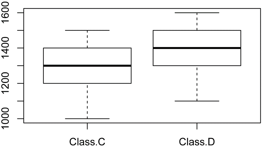
In this example, the SAT scores differ by 100 points between classes, but because the variability is greater than in the previous example, the p-value is not significant.
Class.C = c(1000, 1100, 1200, 1250, 1300, 1300, 1400, 1400, 1450,
1500)
Class.D = c(1100, 1200, 1300, 1350, 1400, 1400, 1500, 1500, 1550, 1600)
t.test(Class.C, Class.D)
Welch Two Sample t-test
t = -1.4174, df = 18, p-value = 0.1735
mean of x mean of y
1290 1390
boxplot(cbind(Class.C, Class.D))
p-values and sample sizes
It should also be remembered that p-values are affected by sample size. For a given effect size and variability in the data, as the sample size increases, the p-value is likely to decrease. For large data sets, small effects can result in significant p-values.
As an example, let’s take the data from Class.C and Class.D and double the number of observations for each without changing the distribution of the values in each, and rename them Class.E and Class.F.
Class.E = c(1000, 1100, 1200, 1250, 1300, 1300, 1400, 1400, 1450,
1500,
1000, 1100, 1200, 1250, 1300, 1300, 1400, 1400, 1450, 1500)
Class.F = c(1100, 1200, 1300, 1350, 1400, 1400, 1500, 1500, 1550, 1600,
1100, 1200, 1300, 1350, 1400, 1400, 1500, 1500, 1550, 1600)
t.test(Class.E, Class.F)
Welch Two Sample t-test
t = -2.0594, df = 38, p-value = 0.04636
mean of x mean of y
1290 1390
boxplot(cbind(Class.E, Class.F))
Notice that the p-value is lower for the t-test for Class.E and Class.F than it was for Class.C and Class.D. Also notice that the means reported in the output are the same, and the box plots would look the same.
Effect size statistics
One way to account for the effect of sample size on our statistical tests is to consider effect size statistics. These statistics reflect the size of the effect in a standardized way, and are unaffected by sample size.
An appropriate effect size statistic for a t-test is Cohen’s d. It takes the difference in means between the two groups and divides by the pooled standard deviation of the groups. Cohen’s d equals zero if the means are the same, and increases to infinity as the difference in means increases relative to the standard deviation.
In the following, note that Cohen’s d is not affected by the sample size difference in the Class.C / Class.D and the Class.E / Class.F examples.
library(lsr)
cohensD(Class.C, Class.D,
method = "raw")
[1] 0.668
cohensD(Class.E, Class.F,
method = "raw")
[1] 0.668
Effect size statistics are standardized so that they are not affected by the units of measurements of the data. This makes them interpretable across different situations, or if the reader is not familiar with the units of measurement in the original data. A Cohen’s d of 1 suggests that the two means differ by one pooled standard deviation. A Cohen’s d of 0.5 suggests that the two means differ by one-half the pooled standard deviation.
For example, if we create new variables—Class.G and Class.H—that are the SAT scores from the previous example expressed as a proportion of a 1600 score, Cohen’s d will be the same as in the previous example.
Class.G = Class.E / 1600
Class.H = Class.F / 1600
Class.G
Class.H
cohensD(Class.G, Class.H,
method="raw")
[1] 0.668
Good practices for statistical analyses
Statistics is not like a trial
When analyzing data, the analyst should not approach the task as would a lawyer for the prosecution. That is, the analyst should not be searching for significant effects and tests, but should instead be like an independent investigator using lines of evidence to find out what is most likely to true given the data, graphical analysis, and statistical analysis available.
The problem of multiple p-values
One concept that will be in important in the following discussion is that when there are multiple tests producing multiple p-values, that there is an inflation of the Type I error rate. That is, there is a higher chance of making false-positive errors.
This simply follows mathematically from the definition of alpha. If we allow a probability of 0.05, or 5% chance, of making a Type I error for any one test, as we do more and more tests, the chances that at least one of them having a false positive becomes greater and greater.
p-value adjustment
One way we deal with the problem of multiple p-values in statistical analyses is to adjust p-values when we do a series of tests together (for example, if we are comparing the means of multiple groups).
Don’t use Bonferroni adjustments
There are various p-value adjustments available in R. In some cases, we will use FDR, which stands for false discovery rate, and in R is an alias for the Benjamini and Hochberg method. There are also cases in which we’ll use Tukey range adjustment to correct for the family-wise error rate.
Unfortunately, students in analysis of experiments courses often learn to use Bonferroni adjustment for p-values. This method is simple to do with hand calculations, but is excessively conservative in most situations, and, in my opinion, antiquated.
There are other p-value adjustment methods, and the choice of which one to use is dictated either by which are common in your field of study, or by doing enough reading to understand which are statistically most appropriate for your application.
Preplanned tests
The statistical tests covered in this book assume that tests are preplanned for their p-values to be accurate. That is, in theory, you set out an experiment, collect the data as planned, and then say “I’m going to analyze it with kind of model and do these post-hoc tests afterwards”, and report these results, and that’s all you would do.
Some authors emphasize this idea of preplanned tests. In contrast is an exploratory data analysis approach that relies upon examining the data with plots and using simple tests like correlation tests to suggest what statistical analysis makes sense.
If an experiment is set out in a specific design, then usually it is appropriate to use the analysis suggested by this design.
p-value hacking
It is important when approaching data from an exploratory approach, to avoid committing p-value hacking. Imagine the case in which the researcher collects many different measurements across a range of subjects. The researcher might be tempted to simply try different tests and models to relate one variable to another, for all the variables. He might continue to do this until he found a test with a significant p-value.
But this would be a form of p-value hacking.
Because an alpha value of 0.05 allows us to make a false-positive error five percent of the time, finding one p-value below 0.05 after several successive tests may simply be due to chance.
Some forms of p-value hacking are more egregious. For example, if one were to collect some data, run a test, and then continue to collect data and run tests iteratively until a significant p-value is found.
Publication bias
A related issue in science is that there is a bias to publish, or to report, only significant results. This can also lead to an inflation of the false-positive rate. As a hypothetical example, imagine if there are currently 20 similar studies being conducted testing a similar effect—let’s say the effect of glucosamine supplements on joint pain. If 19 of those studies found no effect and so were discarded, but one study found an effect using an alpha of 0.05, and was published, is this really any support that glucosamine supplements decrease joint pain?
Clarification of terms and reporting on assignments
"Statistically significant"
In the context of this book, the term "significant" means "statistically significant".
Whenever the decision rule finds that p < alpha, the difference in groups, the association, or the correlation under consideration is then considered "statistically significant" or "significant".
No effect size or practical considerations enter into determining whether an effect is “significant” or not. The only exception is that test assumptions and requirements for appropriate data must also be met in order for the p-value to be valid.
What you need to consider:
• The null hypothesis
• p, alpha, and the decision rule,
• Your result. That is, whether the difference in groups, the association, or the correlation is significant or not.
What you should report on your assignments:
• The p-value
• The conclusion, e.g. "There was a significant difference in the mean heights of boys and girls in the class." It is best to preface this with the "reject" or "fail to reject" language concerning your decision about the null hypothesis.
“Size of the effect” / “effect size”
In the context of this book, I use the term "size of the effect" to suggest the use of summary statistics to indicate how large an effect is. This may be, for example the difference in two medians. I try reserve the term “effect size” to refer to the use of effect size statistics. This distinction isn’t necessarily common.
Usually you will consider an effect in relation to the magnitude of measurements. That is, you might look at the difference in medians as a percent of the median of one group or of the global median. Or, you might look at the difference in medians in relation to the range of answers. For example, a one-point difference on a 5-point Likert item. Counts might be expressed as proportions of totals or subsets.
What you should report on assignments:
• The size of the effect. That is, the difference in medians or means, the difference in counts, or the proportions of counts among groups.
• Where appropriate, the size of the effect expressed as a percentage or proportion.
• If there is an effect size statistic—such as r, epsilon-squared, phi, Cramér's V, or Cohen's d—: report this and its interpretation (small, medium, large), and incorporate this into your conclusion.
"Practical" / "Practical importance"
If there is a significant result, the question of practical importance asks if the difference or association is large enough to matter in the real world.
If there is no significant result, the question of practical importance asks if the a difference or association is large enough to warrant another look, for example by running another test with a larger sample size or that controls variability in observations better.
What you should report on assignments:
• Your conclusion as to whether this effect is large enough to be important in the real world.
• The context, explanation, or support to justify your conclusion.
• In some cases you might include considerations that aren't included in the data presented. Examples might include the cost of one treatment over another, including time investment, or whether there is a large risk in selecting one treatment over another (e.g., if people's lives are on the line).
A few of xkcd comics
Significant
Null hypothesis
P-values
Experiments, sampling, and causation
Types of experimental designs
Experimental designs
A true experimental design assigns treatments in a systematic manner. The experimenter must be able to manipulate the experimental treatments and assign them to subjects. Since treatments are randomly assigned to subjects, a causal inference can be made for significant results. That is, we can say that the variation in the dependent variable is caused by the variation in the independent variable.
For interval/ratio data, traditional experimental designs can be analyzed with specific parametric models, assuming other model assumptions are met. These traditional experimental designs include:
• Completely random design
• Randomized complete block design
• Factorial
• Split-plot
• Latin square
Quasi-experiment designs
Often a researcher cannot assign treatments to individual experimental units, but can assign treatments to groups. For example, if students are in a specific grade or class, it would not be practical to randomly assign students to grades or classes. But different classes could receive different treatments (such as different curricula). Causality can be inferred cautiously if treatments are randomly assigned and there is some understanding of the factors that affect the outcome.
Observational studies
In observational studies, the independent variables are not manipulated, and no treatments are assigned. Surveys are often like this, as are studies of natural systems without experimental manipulation. Statistical analysis can reveal the relationships among variables, but causality cannot be inferred. This is because there may be other unstudied variables that affect the measured variables in the study.
Sampling
Good sampling practices are critical for producing good data. In general, samples need to be collected in a random fashion so that bias is avoided.
In survey data, bias is often introduced by a self-selection bias. For example, internet or telephone surveys include only those who respond to these requests. Might there be some relevant difference in the variables of interest between those who respond to such requests and the general population being surveyed? Or bias could be introduced by the researcher selecting some subset of potential subjects, for example only surveying a 4-H program with particularly cooperative students and ignoring other clubs. This is sometimes called “convenience sampling”.
In election forecasting, good pollsters need to account for selection bias and other biases in the survey process. For example, if a survey is done by landline telephone, those being surveyed are more likely to be older than the general population of voters, and so likely to have a bias in their voting patterns.
Plan ahead and be consistent
It is sometimes necessary to change experimental conditions during the course of an experiment. Equipment might fail, or unusual weather may prevent making meaningful measurements.
But in general, it is much better to plan ahead and be consistent with measurements.
Consistency
People sometimes have the tendency to change measurement frequency or experimental treatments during the course of a study. This inevitably causes headaches in trying to analyze data, and makes writing up the results messy. Try to avoid this.
Controls and checks
If you are testing an experimental treatment, include a check treatment that almost certainly will have an effect and a control treatment that almost certainly won’t. A control treatment will receive no treatment and a check treatment will receive a treatment known to be successful. In an educational setting, perhaps a control group receives no instruction on the topic but on another topic, and the check group will receive standard instruction.
Including checks and controls helps with the analysis in a practical sense, since they serve as standard treatments against which to compare the experimental treatments. In the case where the experimental treatments have similar effects, controls and checks allow you say, for example, “Means for the all experimental treatments were similar, but were higher than the mean for control, and lower than the mean for check treatment.”
Include alternate measurements
It often happens that measuring equipment fails or that a certain measurement doesn’t produce the expected results. It is therefore helpful to include measurements of several variables that can capture the potential effects. Perhaps test scores of students won’t show an effect, but a self-assessment question on how much students learned will.
Include covariates
Including additional independent variables that might affect the dependent variable is often helpful in an analysis. In an educational setting, you might assess student age, grade, school, town, background level in the subject, or how well they are feeling that day.
The effects of covariates on the dependent variable may be of interest in itself. But also, including co-variates in an analysis can better model the data, sometimes making treatment effects more clear or making a model better meet model assumptions.
Optional discussion: Alternative methods to the Null Hypothesis Significance Test
The NHST controversy
Particularly in the fields of psychology and education, there has been much criticism of the null hypothesis significance test approach. From my reading, the main complaints against NHST tend to be:
• Students and researchers don’t really understand the meaning
of p-values.
• p-values don’t include important information like
confidence intervals or parameter estimates.
• p-values have properties that may be misleading, for example that they do not represent effect size, and that they change with sample size.
• We often treat an alpha of 0.05 as a magical cutoff value.
Personally, I don’t find these to be very convincing arguments against the NHST approach.
The first complaint is in some sense pedantic: Like so many things, students and researchers learn the definition of p-values at some point and then eventually forget. This doesn’t seem to impact the usefulness of the approach.
The second point has weight only if researchers use only p-values to draw conclusions from statistical tests. As this book points out, one should always consider the size of the effects and practical considerations of the effects, as well present finding in table or graphical form, including confidence intervals or measures of dispersion. There is no reason why parameter estimates, goodness-of-fit statistics, and confidence intervals can’t be included when a NHST approach is followed.
The properties in the third point also don’t count much as criticism if one is using p-values correctly. One should understand that it is possible to have a small effect size and a small p-value, and vice-versa. This is not a problem, because p-values and effect sizes are two different concepts. We shouldn’t expect them to be the same. The fact that p-values change with sample size is also in no way problematic to me. It makes sense that when there is a small effect size or a lot of variability in the data that we need many samples to conclude the effect is likely to be real.
(One case where I think the considerations in the preceding point are commonly problematic is when people use statistical tests to check for the normality or homogeneity of data or model residuals. As sample size increases, these tests are better able to detect small deviations from normality or homoscedasticity. Too many people use them and think their model is inappropriate because the test can detect a small effect size, that is, a small deviation from normality or homoscedasticity).
The fourth point is a good one. It doesn’t make much sense to come to one conclusion if our p-value is 0.049 and the opposite conclusion if our p-value is 0.051. But I think this can be ameliorated by reporting the actual p-values from analyses, and relying less on p-values to evaluate results.
Overall it seems to me that these complaints condemn poor practices that the authors observe: not reporting the size of effects in some manner; not including confidence intervals or measures of dispersion; basing conclusions solely on p-values; and not including important results like parameter estimates and goodness-of-fit statistics.
Alternatives to the NHST approach
Estimates and confidence intervals
One approach to determining statistical significance is to use estimates and confidence intervals. Estimates could be statistics like means, medians, proportions, or other calculated statistics. This approach can be very straightforward, easy for readers to understand, and easy to present clearly.
Bayesian approach
The most popular competitor to the NHST approach is Bayesian inference. Bayesian inference has the advantage of calculating the probability of the hypothesis given the data, which is what we thought we should be doing in the “Wait, does this make any sense?” section above. Essentially it takes prior knowledge about the distribution of the parameters of interest for a population and adds the information from the measured data to reassess some hypothesis related to the parameters of interest. If the reader will excuse the vagueness of this description, it makes intuitive sense. We start with what we suspect to be the case, and then use new data to assess our hypothesis.
One disadvantage of the Bayesian approach is that it is not obvious in most cases what could be used for legitimate prior information. A second disadvantage is that conducting Bayesian analysis is not as straightforward as the tests presented in this book.
References and further reading
[Video] “Understanding statistical inference” from Statistics Learning Center (Dr. Nic). 2015. www.youtube.com/watch?v=tFRXsngz4UQ.
[Video] “Hypothesis tests, p-value” from Statistics Learning Center (Dr. Nic). 2011. www.youtube.com/watch?v=0zZYBALbZgg.
[Video] “Understanding the p-value” from Statistics Learning Center (Dr. Nic). 2011.
www.youtube.com/watch?v=eyknGvncKLw.
[Video] “Important statistical concepts: significance, strength, association, causation” from Statistics Learning Center (Dr. Nic). 2012. www.youtube.com/watch?v=FG7xnWmZlPE.
“Understanding statistical inference” from Dr. Nic. 2015. Learn and Teach Statistics & Operations Research. creativemaths.net/blog/understanding-statistical-inference/.
“Basic concepts of hypothesis testing” in McDonald, J.H. 2014. Handbook of Biological Statistics. www.biostathandbook.com/hypothesistesting.html.
“Hypothesis testing”, section 4.3, in Diez, D.M., C.D. Barr , and M. Çetinkaya-Rundel. 2012. OpenIntro Statistics, 2nd ed. www.openintro.org/.
“Hypothesis Testing with One Sample”, sections 9.1–9.2 in Openstax. 2013. Introductory Statistics. openstax.org/textbooks/introductory-statistics.
"Proving causation" from Dr. Nic. 2013. Learn and Teach Statistics & Operations Research. creativemaths.net/blog/proving-causation/.
[Video] “Variation and Sampling Error” from Statistics Learning Center (Dr. Nic). 2014. www.youtube.com/watch?v=y3A0lUkpAko.
[Video] “Sampling: Simple Random, Convenience, systematic, cluster, stratified” from Statistics Learning Center (Dr. Nic). 2012. www.youtube.com/watch?v=be9e-Q-jC-0.
“Confounding variables” in McDonald, J.H. 2014. Handbook of Biological Statistics. www.biostathandbook.com/confounding.html.
“Overview of data collection principles”, section 1.3, in Diez, D.M., C.D. Barr , and M. Çetinkaya-Rundel. 2012. OpenIntro Statistics, 2nd ed. www.openintro.org/.
“Observational studies and sampling strategies”, section 1.4, in Diez, D.M., C.D. Barr , and M. Çetinkaya-Rundel. 2012. OpenIntro Statistics, 2nd ed. www.openintro.org/.
“Experiments”, section 1.5, in Diez, D.M., C.D. Barr , and M. Çetinkaya-Rundel. 2012. OpenIntro Statistics, 2nd ed. www.openintro.org/.
Exercises F
1. Which of the following pair is the null hypothesis?
A) The number of heads from the coin is not different from the
number of tails.
B) The number of heads from the coin is different from the number of tails.
2. Which of the following pair is the null hypothesis?
A) The height of boys is different than the height of girls.
B) The height of boys is not different than the height of
girls.
3. Which of the following pair is the null hypothesis?
A) There is an association between classroom and sex. That is,
there is a difference in counts of girls and boys between the classes.
B) There is no association between classroom and sex. That is, there is no difference in counts of girls and boys between the classes.
4. We flip a coin 10 times and it lands on heads 7 times. We want to know if the coin is fair.
a. What is the null hypothesis?
b. Looking at the code below, and assuming an alpha of 0.05,
What do you decide (use the reject or fail to reject language)?
c. In practical terms, what do you conclude?
binom.test(7, 10, 0.5)
Exact binomial test
number of successes = 7, number of trials = 10, p-value = 0.3438
5. We measure the height of 9 boys and 9 girls in a class, in centimeters. We want to know if one group is taller than the other.
a. What is the null hypothesis?
b. Looking at the code below, and assuming an alpha of 0.05,
What do you decide (use the reject or fail to reject language)?
c. In practical terms, what do you conclude? Address the practical importance of the results.
Girls = c(152, 150, 140, 160, 145, 155, 150, 152, 147)
Boys = c(144, 142, 132, 152, 137, 147, 142, 144, 139)
t.test(Girls, Boys)
Welch Two Sample t-test
t = 2.9382, df = 16, p-value = 0.009645
mean of x mean of y
150.1111 142.1111
mean(Boys)
sd(Boys)
quantile(Boys)
mean(Girls)
sd(Girls)
quantile(Girls)
boxplot(cbind(Girls, Boys))
6. We count the number of boys and girls in two classrooms. We are interested to know if there is an association between the classrooms and the number of girls and boys. That is, does the proportion of boys and girls differ statistically across the two classrooms?
a. What is the null hypothesis?
b. Looking at the code below, and assuming an alpha of 0.05,
What do you decide (use the reject or fail to reject language)?
c. In practical terms, what do you conclude?
Classroom Girls Boys
A 13 7
B 5 15
Input =("
Classroom Girls Boys
A 13 7
B 5 15
")
Matrix = as.matrix(read.table(textConnection(Input),
header=TRUE,
row.names=1))
fisher.test(Matrix)
Fisher's Exact Test for Count Data
p-value = 0.02484
Matrix
rowSums(Matrix)
colSums(Matrix)
prop.table(Matrix,
margin=1)
### Proportions for each row
barplot(t(Matrix),
beside = TRUE,
legend = TRUE,
ylim = c(0, 25),
xlab = "Class",
ylab = "Count")
7. Why should you not rely solely on p-values to make a decision in the real world? (You should have at least two reasons.)
8. Create your own example to show the importance of considering the size of the effect. Describe the scenario: what the research question is, and what kind of data were collected. You may make up data and provide real results, or report hypothetical results.
9. Create your own example to show the importance of weighing other practical considerations. Describe the scenario: what the research question is, what kind of data were collected, what statistical results were reached, and what other practical considerations were brought to bear.
10. What is 5e-4 in common decimal notation?