![[banner]](images/banner.jpg "Cohansey River, Fairfield, New Jersey")
Introduction
Proportion data
In general, common parametric tests like t-test and anova shouldn’t be used when the dependent variable is proportion data, since proportion data is by its nature bound at 0 and 1, and is often not normally distributed or homoscedastic.
Data of proportions, percentages, and rates can be thought of as falling into a few different categories.
Proportion data of discrete counts
Some proportion data is derived from discrete counts of “successes” and “failures”, where the “successes” are divided by the total counts. The example below with passing and failing counts across classes is an example of this. Each observation is a percentage from 0 to 100%, or a proportion from 0 to 1. This kind of data can be analyzed with beta regression or can be analyzed with logistic regression.
Proportion data that is inherently proportional
Other proportion data is inherently proportional, in that it’s not possible to count “successes” or “failures”, but instead is derived, for example, by dividing one continuous variable by a given denominator value. The sodium intake example below is an example of this. Another case of this kind of proportion data is when a proportion is assessed by subjective measurement. For example, rating a diseased lawn subjectively on the area dead, such as “this plot is 10% dead, and this plot is 20% dead”. Each observation is a percentage from 0 to 100%, or a proportion from 0 to 1. This kind of data can be analyzed with beta regression.
Rates with different numerators and denominators
Some rates are expressed with numerators and denominators of different measurements or units. For example, the number of cases of a disease per 100,000 people or the number of televisions per student’s home. In these cases, the values are not limited to between 0 and 1, and beta regression is not appropriate.
If the numerator can be considered a count variable, Poisson regression or other methods for count data are usually suggested. As a complication, often the denominator varies in value. For example, if the count is disease occurrence in a city and the denominator is the population in a city. (Each city has a different population.) Or if the numerator is the count of televisions in the home and the denominator is the number of students in the home. In these cases, Poisson regression or related methods are often recommended with an offset for the value in the denominator. These examples are not explored further here, but an example model would be
glm(Count_of_televisions ~ Independent_variable +
offset(log(Number_of_students_in_home)),
family="poisson",
data=Data)
Beta regression
Beta regression can be conducted with the betareg function in the betareg package (Cribari-Neto and Zeileis, 2010). With this function, the dependent variable varies between 0 and 1, but no observation can equal exactly zero or exactly one. The model assumes that the data follow a beta distribution.
p-value and pseudo R-squared for the model
The summary function in betareg produces a pseudo R-squared value for the model, and the recommended test for the p-value for the model is the lrtest function in the lmtest package.
The nagelkerke function in the rcompanion package also works with beta regression objects. The likelihood ratio test there appears to work fine, but the results for pseudo R-squared may be squirrelly, and probably should not be relied upon.
Anova-like table
An anova-like table for factor terms can be produced with the joint_tests function in the emmeans package. It is recommended that the documentation for this function be read before using it.
If this approach doesn’t satisfy the needs of the analyst, nested models can be compared with the lrtest function.
At the time of writing, it appears that the Anova function in the car package works correctly with betareg models, but I didn’t test this extensively. These models are not mentioned explicitly in the car package documentation.
Final note
Note that model assumptions and pitfalls of this approach are not discussed here. The reader is urged to understand the assumptions of this kind of modeling before proceeding.
Packages used in this chapter
The packages used in this chapter include:
• pysch
• betareg
• lmtest
• car
• rcompanion
• multcompView
• emmeans
• ggplot2
The following commands will install these packages if they are not already installed:
if(!require(psych)){install.packages("psych")}
if(!require(betareg)){install.packages("betareg")}
if(!require(lmtest)){install.packages("lmtest")}
if(!require(car)){install.packages("car")}
if(!require(rcompanion)){install.packages("rcompanion")}
if(!require(multcompView)){install.packages("multcompView")}
if(!require(emmeans)){install.packages("emmeans")}
if(!require(ggplot2)){install.packages("ggplot2")}
Beta regression example with discrete counts
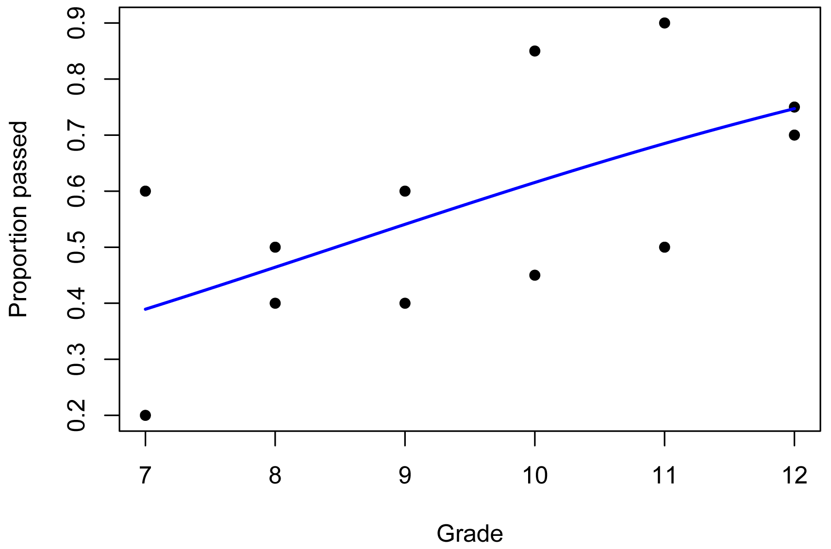
The following example uses counts of students passing or failing an exam, and asks if there is a relationship between the proportion of passing students and Grade. Note that Grade is treated as a numeric variable in this analysis.
Data = read.table(header=TRUE, stringsAsFactors=TRUE, text="
Class Grade Pass Fail
'Bully Hill' 12 14 6
'Keuka Lake' 12 15 5
'Heron Hill' 11 18 2
'Castel Grisch' 11 10 10
'Red Newt' 10 17 3
'Finger Lakes' 10 9 11
'Bellview' 9 12 8
'Auburn Road' 9 8 12
'Balic' 8 10 10
'Cape May' 8 8 12
'Hawk Haven' 7 12 8
'Natali' 7 4 16
")
### Create the proportion variable
Data$Proportion = Data$Pass / (Data$Pass + Data$Fail)
### Check the data frame
library(psych)
headTail(Data)
str(Data)
summary(Data)
Class Grade Pass Fail Proportion
1 Bully Hill 12 14 6 0.7
2 Keuka Lake 12 15 5 0.75
3 Heron Hill 11 18 2 0.9
4 Castel Grisch 11 10 10 0.5
... <NA> ... ... ... ...
9 Balic 8 10 10 0.5
10 Cape May 8 8 12 0.4
11 Hawk Haven 7 12 8 0.6
12 Natali 7 4 16 0.2
Beta regression example
library(betareg)
model.beta = betareg(Proportion ~ Grade, data=Data)library(lmtest)
lrtest(model.beta)
Likelihood ratio test
#Df LogLik Df Chisq Pr(>Chisq)
1 3 5.9273
2 2 2.9897 -1 5.8752 0.01536 *
summary(model.beta)
Pseudo R-squared: 0.3785
library(emmeans)
joint_tests(model.beta)
model term df1 df2 F.ratio p.value
Grade 1 Inf 7.580 0.0059
library(car)
Anova(model.beta)
Analysis of Deviance Table (Type II tests)
Response: Proportion
Df Chisq Pr(>Chisq)
Grade 1 7.3314 0.006776 **
library(rcompanion)
plotPredy(data = Data,
y = Proportion,
x = Grade,
model = model.beta,
xlab = "Grade",
ylab = "Proportion passed")
plot(fitted(model.beta),
residuals(model.beta))
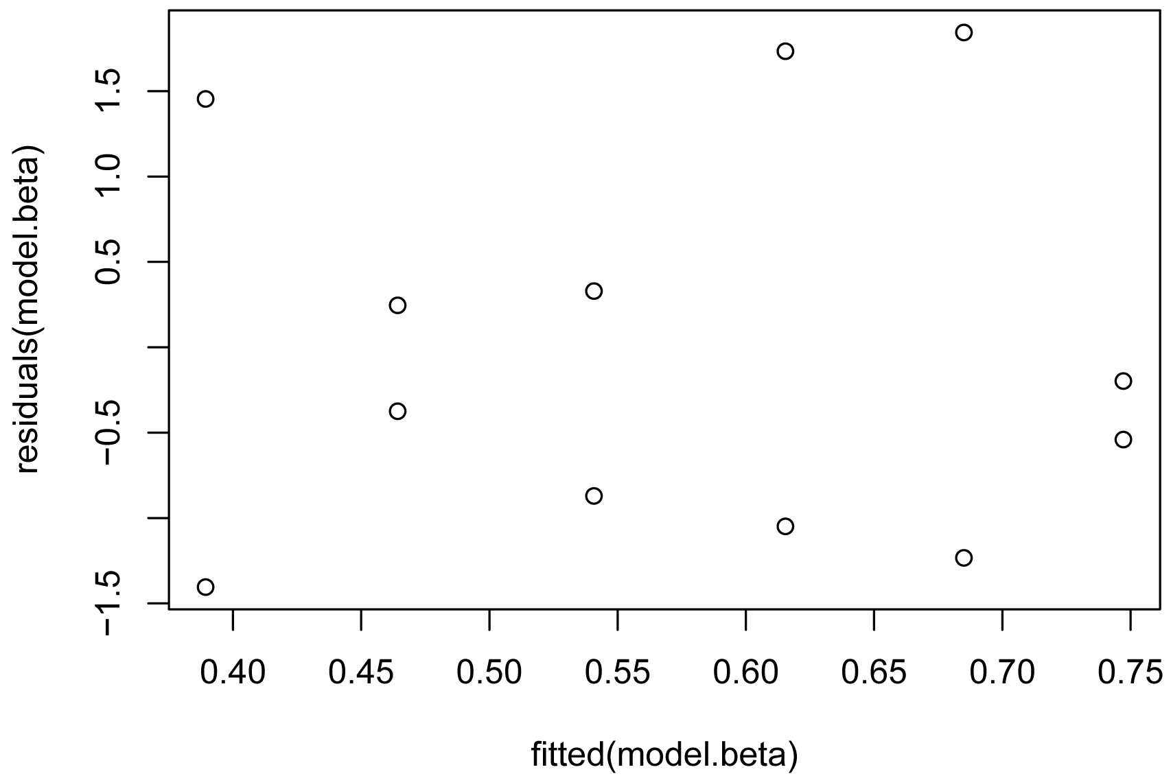
### More diagnostic plots: plot(model.beta)
Alternate logistic regression
Trials = cbind(Data$Pass, Data$Fail) # Successes,
Failures
model.log = glm(Trials ~ Grade,
data = Data,
family = binomial(link="logit"))
library(car)
Anova(model.log,
type="II",
test="Wald")
Analysis of Deviance Table (Type II tests)
Df Chisq Pr(>Chisq)
Grade 1 14.305 0.0001554 ***
library(rcompanion)
nagelkerke(model.log)
$Pseudo.R.squared.for.model.vs.null
Pseudo.R.squared
McFadden 0.190924
Cox and Snell (ML) 0.717212
Nagelkerke (Cragg and Uhler) 0.718174
$Likelihood.ratio.test
Df.diff LogLik.diff Chisq p.value
-1 -7.5784 15.157 9.8946e-05
library(rcompanion)
plotPredy(data = Data,
y = Percent,
x = Grade,
model = model.log,
type = "response", # Needed
for logistic regression
xlab = "Grade",
ylab = "Proportion passing")
plot(fitted(model.beta),
residuals(model.beta))
### More diagnostic plots: plot(model.beta)
Beta regression example with inherently proportional data
This example revisits the data set from the chapter on two-way analysis of variance. Here, the dependent variable Proportion is created by dividing daily student sodium intake by the US FDA “upper safe limit” of 2300 mg. The rest of the analysis is analogous to that of a two-way ANOVA.
Note that for this kind of data, Proportion could be greater than 1, if the observed sodium intake were greater than the 2300 mg limit. Because of this, beta regression may not be the best choice of analysis for this kind of data. Usually, beta regression is used for data that are actually bounded at 0 and 1.
Data = read.table(header=TRUE, stringsAsFactors=TRUE, text="
Instructor Supplement Sodium
'Brendon Small' A 1200
'Brendon Small' A 1400
'Brendon Small' A 1350
'Brendon Small' A 950
'Brendon Small' A 1400
'Brendon Small' B 1150
'Brendon Small' B 1300
'Brendon Small' B 1325
'Brendon Small' B 1425
'Brendon Small' B 1500
'Brendon Small' C 1250
'Brendon Small' C 1150
'Brendon Small' C 950
'Brendon Small' C 1150
'Brendon Small' C 1600
'Brendon Small' D 1300
'Brendon Small' D 1050
'Brendon Small' D 1300
'Brendon Small' D 1700
'Brendon Small' D 1300
'Coach McGuirk' A 1100
'Coach McGuirk' A 1200
'Coach McGuirk' A 1250
'Coach McGuirk' A 1050
'Coach McGuirk' A 1200
'Coach McGuirk' B 1250
'Coach McGuirk' B 1350
'Coach McGuirk' B 1350
'Coach McGuirk' B 1325
'Coach McGuirk' B 1525
'Coach McGuirk' C 1225
'Coach McGuirk' C 1125
'Coach McGuirk' C 1000
'Coach McGuirk' C 1125
'Coach McGuirk' C 1400
'Coach McGuirk' D 1200
'Coach McGuirk' D 1150
'Coach McGuirk' D 1400
'Coach McGuirk' D 1500
'Coach McGuirk' D 1200
'Melissa Robins' A 900
'Melissa Robins' A 1100
'Melissa Robins' A 1150
'Melissa Robins' A 950
'Melissa Robins' A 1100
'Melissa Robins' B 1150
'Melissa Robins' B 1250
'Melissa Robins' B 1250
'Melissa Robins' B 1225
'Melissa Robins' B 1325
'Melissa Robins' C 1125
'Melissa Robins' C 1025
'Melissa Robins' C 950
'Melissa Robins' C 925
'Melissa Robins' C 1200
'Melissa Robins' D 1100
'Melissa Robins' D 950
'Melissa Robins' D 1300
'Melissa Robins' D 1400
'Melissa Robins' D 1100
")
### Order factors by the order in data frame
### Otherwise, R will alphabetize them
Data$Instructor = factor(Data$Instructor,
levels=unique(Data$Instructor))
Data$Supplement = factor(Data$Supplement,
levels=unique(Data$Supplement))
### Create proportion variable
Data$Proportion = Data$Sodium / 2300
### Check the data frame
library(psych)
headTail(Data)
str(Data)
summary(Data)
Instructor Supplement Sodium Proportion
1 Brendon Small A 1200 0.52
2 Brendon Small A 1400 0.61
3 Brendon Small A 1350 0.59
4 Brendon Small A 950 0.41
... <NA> <NA> ... ...
57 Melissa Robins D 950 0.41
58 Melissa Robins D 1300 0.57
59 Melissa Robins D 1400 0.61
60 Melissa Robins D 1100 0.48
Beta regression
library(betareg)
model = betareg(Proportion ~ Instructor + Supplement + Instructor:Supplement,
data = Data)
library(emmeans)
joint_tests(model)
model term df1 df2 F.ratio p.value
Instructor 2 Inf 7.535 0.0005
Supplement 3 Inf 5.169 0.0014
Instructor:Supplement 6 Inf 0.207 0.9748
library(car)
Anova(model)
Analysis of Deviance Table (Type II tests)
Df Chisq Pr(>Chisq)
Instructor 2 14.9873 0.0005566 ***
Supplement 3 15.3766 0.0015216 **
Instructor:Supplement 6 1.1985 0.9769603
library(lmtest)
lrtest(model)
Likelihood ratio test
#Df LogLik Df Chisq Pr(>Chisq)
1 13 82.956
2 2 70.260 -11 25.392 0.007984 **
summary(model)
Pseudo R-squared: 0.3431
plot(fitted(model),
residuals(model))
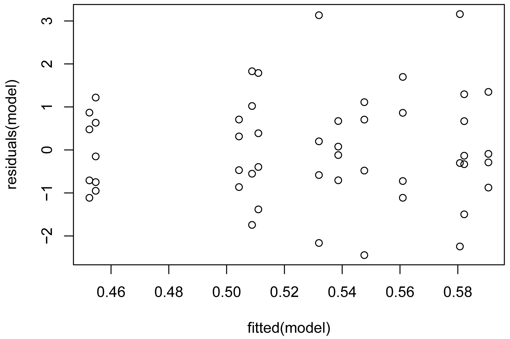
### More diagnostic plots: plot(model)
library(multcompView)
library(emmeans)
marginal = emmeans(model,
~ Instructor)
pairs(marginal,
adjust="tukey")
Sum = cld(marginal,
alpha = 0.05,
Letters = letters, ### Use
lowercase letters for .group
adjust = "tukey") ###
Tukey-adjusted comparisons
Sum
Instructor emmean SE df asymp.LCL asymp.UCL .group
Melissa Robins 0.4886613 0.01361908 NA 0.4561425 0.5211801 a
Coach McGuirk 0.5417084 0.01357579 NA 0.5092930 0.5741238 b
Brendon Small 0.5606374 0.01354438 NA 0.5282970 0.5929779 b
Results are averaged over the levels of: Supplement
Confidence level used: 0.95
Conf-level adjustment: sidak method for 3 estimates
P value adjustment: tukey method for comparing a family of 3 estimates
significance level used: alpha = 0.05
### Order data frame for plotting
Sum = Sum[order(factor(Sum$Instructor,
levels=c("Brendon Small",
"Coach McGuirk",
"Melissa Robins"))),]
Sum
Instructor emmean SE df asymp.LCL asymp.UCL .group
Brendon Small 0.5606374 0.01354438 NA 0.5282970 0.5929779 b
Coach McGuirk 0.5417084 0.01357579 NA 0.5092930 0.5741238 b
Melissa Robins 0.4886613 0.01361908 NA 0.4561425 0.5211801 a
library(ggplot2)
ggplot(Sum, ### The data frame to
use.
aes(x = Instructor,
y = emmean)) +
geom_errorbar(aes(ymin = asymp.LCL,
ymax = asymp.UCL),
width = 0.05,
size = 0.5) +
geom_point(shape = 15,
size = 4) +
theme_bw() +
theme(axis.title = element_text(face = "bold")) +
ylab("EM mean proportion of sodium intake") +
annotate("text",
x = 1:3,
y = Sum$asymp.UCL + 0.008,
label = gsub(" ", "", Sum$.group))

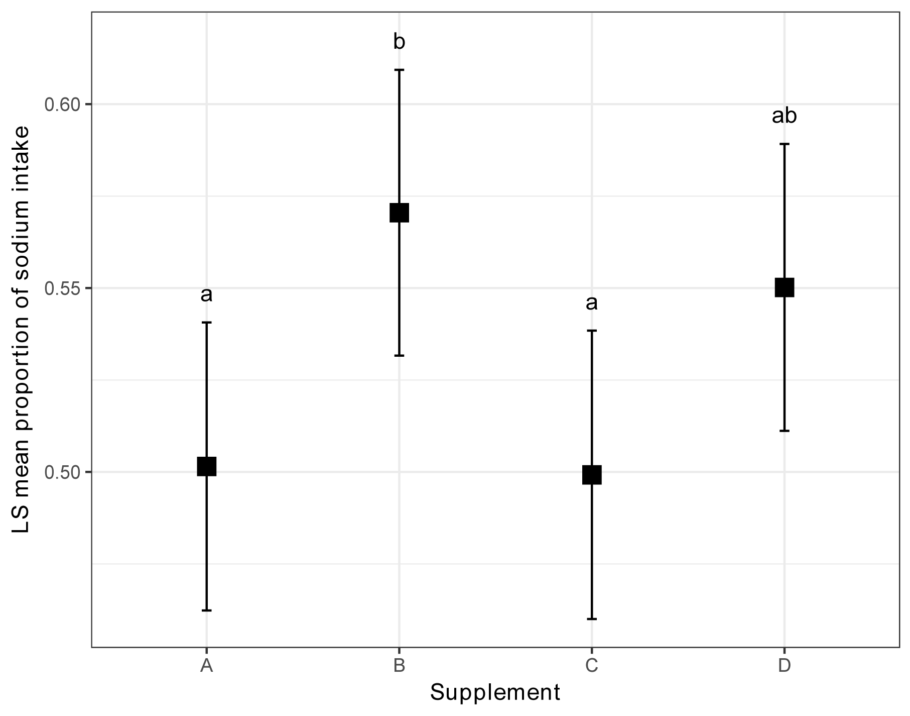
marginal = emmeans(model,
~ Supplement)
pairs(marginal,
adjust="tukey")
Sum = cld(marginal,
alpha = 0.05,
Letters = letters, ### Use
lowercase letters for .group
adjust = "tukey") ###
Tukey-adjusted comparisons
Sum
### Order data frame for plotting
Sum = Sum[order(factor(Sum$Supplement,
levels=c("A", "B", "C",
"D"))),]
Sum
library(ggplot2)
ggplot(Sum, ### The data frame to
use.
aes(x = Supplement,
y = emmean)) +
geom_errorbar(aes(ymin = asymp.LCL,
ymax = asymp.UCL),
width = 0.05,
size = 0.5) +
geom_point(shape = 15,
size = 4) +
theme_bw() +
theme(axis.title = element_text(face = "bold")) +
ylab("EM mean proportion of sodium intake") +
annotate("text",
x = 1:4,
y = Sum$asymp.UCL + 0.008,
label = gsub(" ", "", Sum$.group))
References
Cribari-Neto, F. and Zeileis, A. 2010. Beta Regression in R. Journal of Statistical Software 34(2). www.jstatsoft.org/index.php/jss/article/download/v034i02/378.