![[banner]](images/banner.jpg "Cohansey River, Fairfield, New Jersey")
An assumption of many statistical tests is that observations are independent of one another. This means that the value for one observation is unlikely to be influenced by the value of another observation. If we pick students at random from a class and measure their height, we can assume the height of the first student will not affect the height of the next student. These observations would be independent. If, however, we measured the height of the same students across years, we would expect that a student who is tall this year would likely be tall the next, and so on. These observations would not be independent. We might call this second set of observations non-independent, paired, dependent, or correlated.
Dependent samples commonly arise in a few situations. One is repeated measures, in which the same subject is measured on multiple dates. This is like the student height example described above.
A second is when we are taking multiple measurements of the same individual. An example of this might be if we are testing students on multiple concepts; we might suspect that if a student scores well in one section, that she is likely to score well in the other sections. Another example would be measuring the length of people’s hands. We would suspect that someone with a large left hand is likely to have a large right hand. A final example would be if student raters were measuring multiple instructors. We might suspect that a rater who scores one instructor low might be likely to score another instructor low.
A related concept is that of blocks. If observations can be broken into meaningful groups where values are likely to be different, this should be taken into account. For example, if we are measuring students’ scores from two classes, and we suspect scores would be lower for one class than the other. If we were testing instructional methods, we may care about the effect of the instructional methods, and not care at all about the classes per se, but we want to take differences due to the different classes into account.
Packages used in this chapter
The packages used in this chapter include:
• FSA
• rcompanion
The following commands will install these packages if they are not already installed:
if(!require(FSA)){install.packages("FSA")}
if(!require(rcompanion)){install.packages("rcompanion")}
An example of paired and unpaired data
In this example we measure the length in centimeters of both the left hand and the right hand for each of 16 individuals.
Data = read.table(header=TRUE, stringsAsFactors=TRUE, text="
Individual Hand Length
A Left 17.5
B Left 18.4
C Left 16.2
D Left 14.5
E Left 13.5
F Left 18.9
G Left 19.5
H Left 21.1
I Left 17.8
J Left 16.8
K Left 18.4
L Left 17.3
M Left 18.9
N Left 16.4
O Left 17.5
P Left 15.0
A Right 17.6
B Right 18.5
C Right 15.9
D Right 14.9
E Right 13.7
F Right 18.9
G Right 19.5
H Right 21.5
I Right 18.5
J Right 17.1
K Right 18.9
L Right 17.5
M Right 19.5
N Right 16.5
O Right 17.4
P Right 15.6
")
### Note: for the paired test below, data must
be ordered so that
### the first observation of Group 1
### is the same subject as the first observation of Group 2
### The following will order the data frame by Hand, and then by Individual
Data = Data[order(Data$Hand, Data$Individual),]
### Check the data frame
Data
str(Data)
summary(Data)
Box plot and summary statistics by group
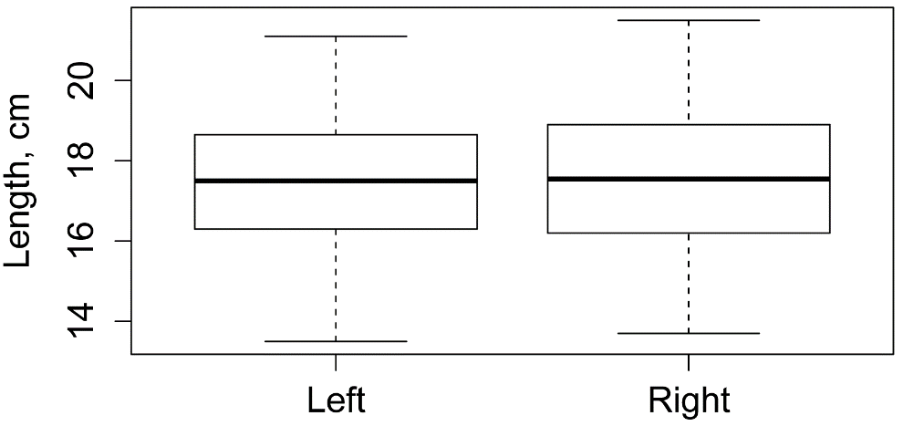
Below, the descriptive statistics suggest that left hands and right hands had similar means, medians, and standard deviations for Length.
library(FSA)
Summarize(Length ~ Hand,
data=Data,
digits=3)
boxplot(Length ~ Hand,
data=Data,
ylab="Length, cm")
Hand n mean sd min Q1 median Q3 max percZero
1 Left 16 17.356 1.948 13.5 16.35 17.50 18.52 21.1 0
2 Right 16 17.594 1.972 13.7 16.35 17.55 18.90 21.5 0
Bar plot to show paired differences
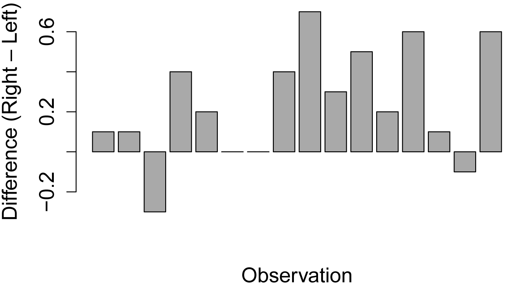
The previous summary statistics, however, do not capture the paired nature of the data. Instead, we want to investigate the difference between left hand and right hand for each individual. We can calculate this difference, and use a bar plot to visualize the difference. For most observations, the right hand was larger, with Right – Left being greater than zero.
Left_hand = Data$Length[Data$Hand=="Left"]
Right_hand = Data$Length[Data$Hand=="Right"]
Difference = Right_hand - Left_hand
barplot(Difference,
col="dark gray",
xlab="Observation",
ylab="Difference (Right – Left)")
Paired t-test and unpaired t-test
t-tests are discussed later in this book. It isn’t important that you understand the test fully at this point. In this example, a t-test that ignores the pairing of observations found no difference between the mean length for left hand and right hand, whereas the t-test that accounts for the paired observations found a significant difference. On average the right hands were about 0.2 cm longer than their paired left hands.
t.test(Length ~ Hand,
data = Data,
paired = FALSE)
Welch Two Sample t-test
t = -0.3427, df = 29.996, p-value = 0.7342
### No difference between left hand and right if
length treated as not paired
t.test(Length ~ Hand,
data = Data,
paired = TRUE)
Paired t-test
t = -3.3907, df = 15, p-value = 0.004034
mean of the differences
-0.2375
### Significant difference between left hand and
right
### if length treated as paired
Histogram of differences with normal curve
To be sure our paired t-test was valid, we’ll plot the differences in hands to be sure their distribution is approximately normal.
Left_hand = Data$Length[Data$Hand=="Left"]
Right_hand = Data$Length[Data$Hand=="Right"]
Difference = Right_hand - Left_hand
library(rcompanion)
plotNormalHistogram(Difference,
xlab = "Difference")
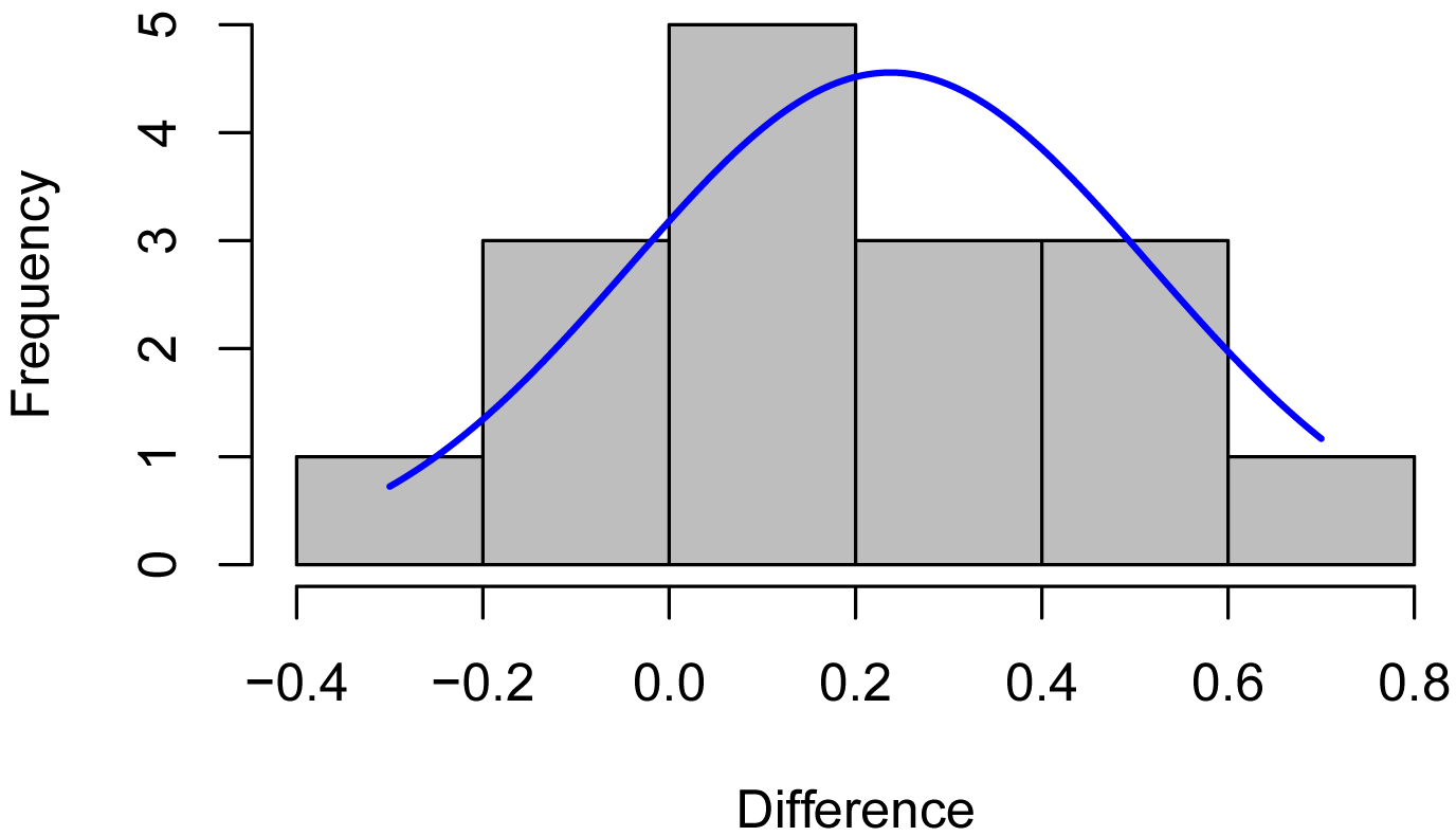
### Distribution of differences is probably close enough to normal
### for paired t-test