![[banner]](images/banner.jpg "Cohansey River, Fairfield, New Jersey")
Packages used in this chapter
The packages used in this chapter include:
• robustbase
• psych
• minpack.lm
• car
• rcompanion
The following commands will install these packages if they are not already installed:
if(!require(robustbase)){install.packages("robustbase")}
if(!require(pysch)){install.packages("pysch")}
if(!require(nlstools)){install.packages("nlstools")}
if(!require(minpack.lm)){install.packages("minpack.lm")}
if(!require(car)){install.packages("car")}
if(!require(rcompanion)){install.packages("rcompanion")}
More complex experimental designs
Except for t-tests, the approach of this book for parametric statistics has been to develop linear models (with the lm function) or mixed effects models (with the nlme or lme4 packages) and then to apply analysis of variance, model checking, and post-hoc testing.
These relatively simple models can be expanded to include more independent variables of either continuous or factor type. Likewise, more complex designs can include nested and crossed factors. Some traditional experimental designs include Latin square, split plot, and incomplete block.
Analysis of co-variance.
Analysis of covariance combines continuous independent variables with factor independent variables.
A related design is the paired watershed design which, while it was developed for watershed studies, can be adapted to various situations in a variety of fields.
“Analysis of Covariance” in Mangiafico, S.S. 2015. An R Companion for the Handbook of Biological Statistics. rcompanion.org/rcompanion/e_04.html.
Clausen, J.C. and J. Spooner. 1993. Paired Watershed Study Design. 841-F-93-009. United States Environmental Protection Agency, Office of Water. Washington, DC. nepis.epa.gov/Exe/ZyPURL.cgi?Dockey=20004PR6.TXT.
Dressing, S.A. and D.W. Meals. 2005. Designing water quality monitoring programs for watershed projects. U.S. Environmental Protection Agency. Fairfax, VA. www.epa.gov/sites/default/files/2015-10/documents/technote2_wq_monitoring.pdf.
Nonlinear regression and curvilinear regression
Nonlinear and curvilinear regression are similar to linear regression, except that the relationship between the dependent variable and the independent variable is curved in some way. Specific methods include polynomial regression, spline regression, and nonlinear regression.
Polynomial regression was covered briefly in the previous chapter, while some examples of curvilinear regression are shown below in the “Linear plateau and quadratic plateau models” section in this chapter.
For further discussion, see:
“Curvilinear Regression” in Mangiafico, S.S. 2015. An R Companion for the Handbook of Biological Statistics. rcompanion.org/rcompanion/e_03.html.
Multiple regression
Multiple regression is similar to linear regression, except that the model contains multiple independent variables.
The polynomial regression example in the previous chapter is one example of multiple regression.
For further discussion, see:
“Multiple Regression” in Mangiafico, S.S. 2015. An R Companion for the Handbook of Biological Statistics. rcompanion.org/rcompanion/e_05.html.
Logistic regression
Logistic regression is similar to linear regression, except that the dependent variable is categorical. In standard logistic regression, the dependent variable has only two levels, and in multinomial logistic regression, the dependent variable can have more than two levels.
For examples of logistic regression, see the chapter Models for Nominal Data in this book.
Analysis of count data
When the dependent variable is a counted quantity and not a measured quantity, it is appropriate to use Poisson regression or related techniques.
For a discussion of when standard parametric approaches may or may not be used with count data, see the “Count data may not be appropriate for common parametric tests” section in the Introduction to Parametric Tests chapter.
For examples of appropriate ways to model count data, see the Regression for Count Data chapter in this book.
Robust techniques
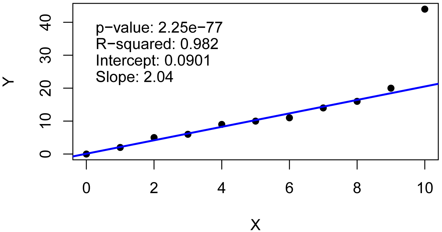
Standard parametric analyses can be sensitive to outliers and other deviations from assumptions of the analyses. The example below shows that a single point can affect the predicted line from standard linear regression. It is said that this point has high leverage, as so has high influence in the model.
One approach in these cases is to use nonparametric techniques.
Another approach is to adjust the model to better fit the data.
A third way is to determine if certain data points are true outliers, and then give them further examination.
A fourth way is to use a robust technique such as robust regression. The references below discuss robust regression and robust techniques appropriate for designs lending themselves to an analysis of variance approach.
“One-way Analysis with Permutation Test” in Mangiafico, S.S. 2015. An R Companion for the Handbook of Biological Statistics. rcompanion.org/rcompanion/d_06a.html.
“Two-way Anova with Robust Estimation” in Mangiafico, S.S. 2015. An R Companion for the Handbook of Biological Statistics. rcompanion.org/rcompanion/d_08a.html.
Search for Robust regression in the following:
“Correlation and Linear Regression” in Mangiafico, S.S. 2015. An R Companion for the Handbook of Biological Statistics. rcompanion.org/rcompanion/e_01.html.
Example of robust linear regression
Note that this example does not include checking assumptions of the model, but is intended only to compare the results of ordinary linear regression and robust regression when there is a data point with high influence.
Data = read.table(header=TRUE, stringsAsFactors=TRUE, text="
X
Y
0 0
1 2
2 5
3 6
4 9
5 10
6 11
7 14
8 16
9 20
10 44
")
Linear regression
model = lm(Y ~ X,
data = Data)
summary(model)
Coefficients:
Estimate Std. Error t value Pr(>|t|)
(Intercept) -3.1364 3.6614 -0.857 0.413888
X 3.1182 0.6189 5.038 0.000701 ***
Residual standard error: 6.491 on 9 degrees of freedom
Multiple R-squared: 0.7383, Adjusted R-squared: 0.7092
F-statistic: 25.39 on 1 and 9 DF, p-value: 0.0007013
Calculate statistics and plot
Pvalue = pf(summary(model)$fstatistic[1],
summary(model)$fstatistic[2],
summary(model)$fstatistic[3],
lower.tail = FALSE)
R2 = summary(model)$r.squared
t1 = paste0("p-value: ", signif(Pvalue, digits=3))
t2 = paste0("R-squared: ", signif(R2, digits=3))
t3 = paste0("Intercept: ", signif(coef(model)[1], digits=3))
t4 = paste0("Slope: ", signif(coef(model)[2], digits=3))
plot(Y ~ X,
data = Data,
pch = 16)
abline(model,
col="blue",
lwd=2)
text(0, 38, labels = t1, pos=4)
text(0, 33, labels = t2, pos=4)
text(0, 28, labels = t3, pos=4)
text(0, 23, labels = t4, pos=4)

Cook’s distance
Cook’s distance is a measure of influence of each data point, specifically determining how much predicted values would change if the observation were deleted. It is sometimes recommended that a Cook’s distance of 1 or more merits further examination of the data point. However, there are other recommendations for critical values for Cook’s distance.
In this case, the high Cook’s distance for observation 11 makes it a candidate for further evaluation.
barplot(cooks.distance(model))

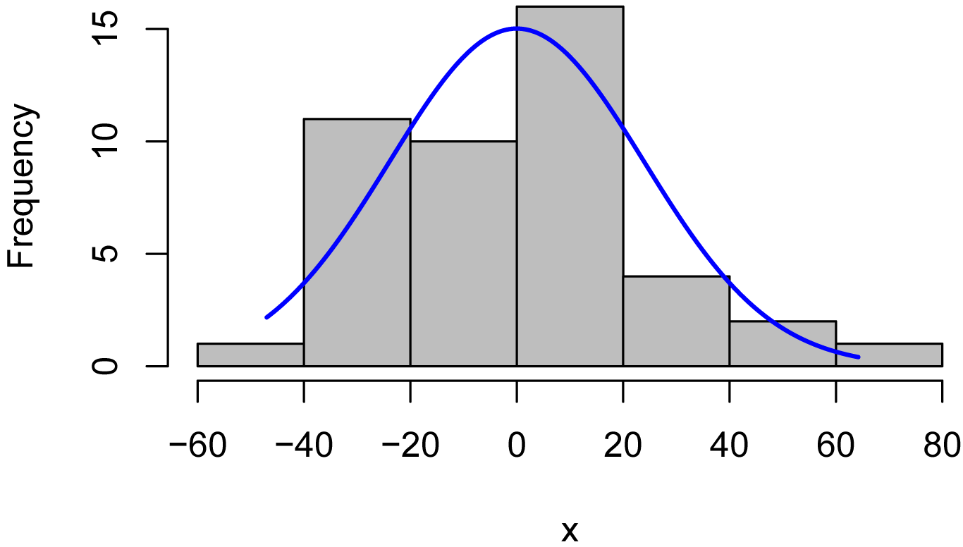
Plot of residuals
This plot suggests that the residuals are not independent of the fitted values. We would probably want to adjust the model by adding additional terms, using a nonlinear or curvilinear approach, or using a robust analysis to minimize the influence of certain data points.
plot(fitted(model),
residuals(model))

Robust regression
library(robustbase)
model.r = lmrob(Y ~ X,
data = Data)
summary(model.r)
Coefficients:
Estimate Std. Error t value Pr(>|t|)
(Intercept) 0.09015 0.32804 0.275 0.79
X 2.04249 0.10970 18.619 1.7e-08 ***
Robust residual standard error: 0.9378
Multiple R-squared: 0.9817, Adjusted R-squared: 0.9796
Calculate statistics and plot
model.null = lmrob(Y ~ 1,
data = Data)
Pvalue = anova(model.r, model.null)[4][2,1]
R2 = summary(model.r)$r.squared
t1 = paste0("p-value: ", signif(Pvalue, digits=3))
t2 = paste0("R-squared: ", signif(R2, digits=3))
t3 = paste0("Intercept: ", signif(coefficients(model.r)[1],
digits=3))
t4 = paste0("Slope: ", signif(coefficients(model.r)[2],
digits=3))
plot(Y ~ X,
data = Data,
pch = 16)
abline(model.r,
col="blue",
lwd=2)
text(0, 38, labels = t1, pos=4)
text(0, 33, labels = t2, pos=4)
text(0, 28, labels = t3, pos=4)
text(0, 23, labels = t4, pos=4)
Kendall Theil nonparametric linear regression
Kendall–Theil regression is a completely nonparametric approach to linear regression. It is robust to outliers in the y values. It simply computes all the lines between each pair of points, and uses the median of the slopes of these lines. This method is sometimes called Theil–Sen. A modified, and preferred, method is named after Siegel.
The mblm function in the mblm package uses the Siegel method by default. The Theil–Sen procedure can be chosen with the repeated=FALSE option. See library(mblm); ?mblm for more details.
Data = read.table(header=TRUE, stringsAsFactors=TRUE, text="
X
Y
0 0
1 2
2 5
3 6
4 9
5 10
6 11
7 14
8 16
9 20
10 44
")
library(mblm)
model = mblm(Y ~ X,
data=Data)
summary(model)
Coefficients:
Estimate MAD V value Pr(>|V|)
(Intercept) 0 0 6 0.78741
X 2 0 66 0.00327 **
Pvalue = as.numeric(summary(model)$coefficients[2,4])
Intercept = as.numeric(summary(model)$coefficients[1,1])
Slope = as.numeric(summary(model)$coefficients[2,1])
R2 = NULL
t1 = paste0("p-value: ", signif(Pvalue, digits=3))
t2 = paste0("R-squared: ", "NULL")
t3 = paste0("Intercept: ", signif(Intercept, digits=3))
t4 = paste0("Slope: ", signif(Slope, digits=3))
plot(Y ~ X,
data = Data,
pch = 16)
abline(model,
col="blue",
lwd=2)
text(1, 40, labels = t1, pos=4)
text(1, 36, labels = t2, pos=4)
text(1, 32, labels = t3, pos=4)
text(1, 28, labels = t4, pos=4)

Contrasts in Linear Models
Contrasts can be used in linear models to compare groups of treatments to one another. For example, if you were testing four curricula and wanted to compare the effect of One and Two vs. Three and Four, you could accomplish this with a single-degree-of freedom contrast.
“Contrasts in Linear Models” in Mangiafico, S.S. 2015. An R Companion for the Handbook of Biological Statistics. rcompanion.org/rcompanion/h_01.html.
Polynomial Contrasts in Linear Models
Polynomial contrasts can be used in linear models to determine if there is a linear or quadratic trend across treatments that are ordinal in nature. For example, with treatments “Zero”, “Low”, “Medium”, “High”, the question of interest may if there is a general linear trend in response across these
“Polynomial Contrasts in Models” in Mangiafico, S.S. 2015. An R Companion for the Handbook of Biological Statistics. rcompanion.org/rcompanion/h_03.html.
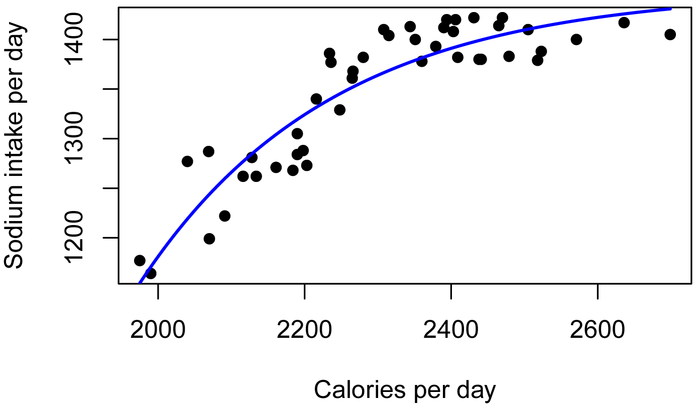
Linear plateau and quadratic plateau models
Linear plateau and quadratic plateau models are segmented models for bivariate data, typically where the y-value increases with an increase in x to some critical value, beyond which the y-value ceases to increase. The statistics of interest include the critical value (the x-value above which there is no further increase in y), and the plateau value (the statistically highest value that y reaches).
For another example of these models, see the “Use the best model” section of the Basic Plots chapter.
Also included in this section is an example of curvilinear regression, with a Mitscherlich–Bray model fit to the same data.
Examples of linear plateau and quadratic plateau models
Data = read.table(header=TRUE, stringsAsFactors=TRUE, text="
Instructor Grade Weight Calories Sodium Score
'Brendon Small' 6 43 2069 1287 77
'Brendon Small' 6 41 1990 1164 76
'Brendon Small' 6 40 1975 1177 76
'Brendon Small' 6 44 2116 1262 84
'Brendon Small' 6 45 2161 1271 86
'Brendon Small' 6 44 2091 1222 87
'Brendon Small' 6 48 2236 1377 90
'Brendon Small' 6 47 2198 1288 78
'Brendon Small' 6 46 2190 1284 89
'Jason Penopolis' 7 45 2134 1262 76
'Jason Penopolis' 7 45 2128 1281 80
'Jason Penopolis' 7 46 2190 1305 84
'Jason Penopolis' 7 43 2070 1199 68
'Jason Penopolis' 7 48 2266 1368 85
'Jason Penopolis' 7 47 2216 1340 76
'Jason Penopolis' 7 47 2203 1273 69
'Jason Penopolis' 7 43 2040 1277 86
'Jason Penopolis' 7 48 2248 1329 81
'Melissa Robins' 8 48 2265 1361 67
'Melissa Robins' 8 46 2184 1268 68
'Melissa Robins' 8 53 2441 1380 66
'Melissa Robins' 8 48 2234 1386 65
'Melissa Robins' 8 52 2403 1408 70
'Melissa Robins' 8 53 2438 1380 83
'Melissa Robins' 8 52 2360 1378 74
'Melissa Robins' 8 51 2344 1413 65
'Melissa Robins' 8 51 2351 1400 68
'Paula Small' 9 52 2390 1412 78
'Paula Small' 9 54 2470 1422 62
'Paula Small' 9 49 2280 1382 61
'Paula Small' 9 50 2308 1410 72
'Paula Small' 9 55 2505 1410 80
'Paula Small' 9 52 2409 1382 60
'Paula Small' 9 53 2431 1422 70
'Paula Small' 9 56 2523 1388 79
'Paula Small' 9 50 2315 1404 71
'Coach McGuirk' 10 52 2406 1420 68
'Coach McGuirk' 10 58 2699 1405 65
'Coach McGuirk' 10 57 2571 1400 64
'Coach McGuirk' 10 52 2394 1420 69
'Coach McGuirk' 10 55 2518 1379 70
'Coach McGuirk' 10 52 2379 1393 61
'Coach McGuirk' 10 59 2636 1417 70
'Coach McGuirk' 10 54 2465 1414 59
'Coach McGuirk' 10 54 2479 1383 61
")
### Order factors by the order in data frame
### Otherwise, R will alphabetize them
Data$Instructor = factor(Data$Instructor,
levels=unique(Data$Instructor))
### Check the data frame
library(psych)
headTail(Data)
str(Data)
summary(Data)
Linear plateau model
The nls function in the native stats package can fit nonlinear and curvilinear functions. To accomplish this, a function—linplat, here—will be defined with the x and y variables (Calories and Sodium) along with parameters (a, b, and clx). It is the goal of the nls function to find the best fit values for these parameters for these data.
The code below starts with an attempt to find reasonable starting values for the parameters. If these starting values don’t yield appropriate results, other starting values can be tried.
The fitted parameters a, b, and clx designate the best fit intercept, slope, and critical x value. The plateau value is calculated as a + b * clx.
### Find reasonable initial values for parameters
fit.lm = lm(Sodium ~ Calories, data=Data)
a.ini = fit.lm$coefficients[1]
b.ini = fit.lm$coefficients[2]
clx.ini = mean(Data$Calories)
### Define linear plateau function
linplat = function(x, a, b, clx)
{ifelse(x < clx, a + b * x,
a + b * clx)}
### Find best fit parameters
model = nls(Sodium ~ linplat(Calories, a, b, clx),
data = Data,
start = list(a = a.ini,
b = b.ini,
clx = clx.ini),
trace = FALSE,
nls.control(maxiter = 1000))
summary(model)
Parameters:
Estimate Std. Error t value Pr(>|t|)
a -128.85535 116.10819 -1.11 0.273
b 0.65768 0.05343 12.31 1.6e-15 ***
clx 2326.51521 16.82086 138.31 < 2e-16 ***
p-value and pseudo R-squared
### Find pseudo R-squared
library(rcompanion)
efronRSquared(model)
EfronRSquared
0.892
### Define null model
nullfunct = function(x, m){m}
m.ini = mean(Data$Sodium)
null = nls(Sodium ~ nullfunct(Calories, m),
data = Data,
start = list(m = m.ini),
trace = FALSE,
nls.control(maxiter = 1000))
### Find p-value and pseudo R-squared
library(rcompanion)
nagelkerke(model,
null)
$Pseudo.R.squared.for.model.vs.null
Pseudo.R.squared
McFadden 0.195417
Cox and Snell (ML) 0.892004
Nagelkerke (Cragg and Uhler) 0.892014
$Likelihood.ratio.test
Df.diff LogLik.diff Chisq p.value
-2 -50.077 100.15 1.785e-22
Determine confidence intervals for parameter estimates
library(nlstools)
confint2(model,
level = 0.95)
2.5 % 97.5 %
a -363.1711583 105.4604611
b 0.5498523 0.7654999
clx 2292.5693351 2360.4610904
library(nlstools)
Boot = nlsBoot(model)
summary(Boot)
------
Bootstrap statistics
Estimate Std. error
a -143.5189740 111.18292997
b 0.6643267 0.05132983
clx 2326.8124177 16.71482729
------
Median of bootstrap estimates and percentile confidence intervals
Median 2.5% 97.5%
a -143.5474796 -376.3224461 73.437548
b 0.6638483 0.5652069 0.771089
clx 2327.1279329 2292.5244830 2363.929178
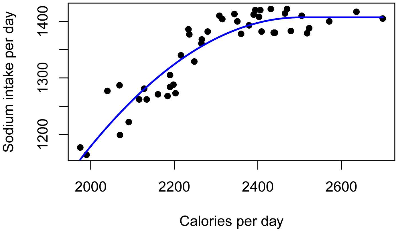
Plot data with best fit line
library(rcompanion)
plotPredy(data = Data,
x = Calories,
y = Sodium,
model = model,
xlab = "Calories per day",
ylab = "Sodium intake per day")

A plot of daily sodium intake vs. daily caloric
intake for students. Best fit linear plateau model is shown. Critical x value
= 2327 calories, and Plateau y = 1401 mg. p < 0.0001. Pseudo R-squared
(Nagelkerke) = 0.892.
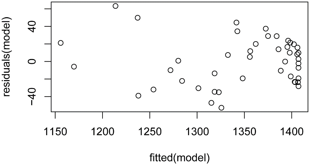
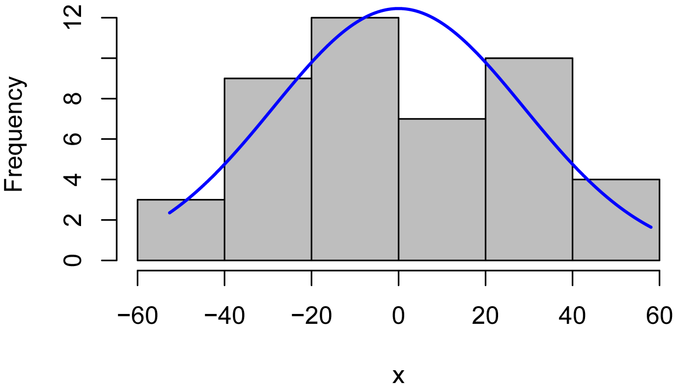
Plots of residuals
x = residuals(model)
library(rcompanion)
plotNormalHistogram(x)
plot(fitted(model),
residuals(model))

Quadratic plateau model
A quadratic plateau model is similar to a linear plateau model, except that the linear segment is replaced with a quadratic function.
The fitted parameters a, b, and clx designate the best fit intercept, linear coefficient, and critical x value. The quadratic coefficient is calculated as –0.5 * b / clx. The plateau value is calculated as a + b * clx –0.5 * b * clx.
### Find reasonable initial values for parameters
fit.lm = lm(Sodium ~ Calories, data=Data)
a.ini = fit.lm$coefficients[1]
b.ini = fit.lm$coefficients[2]
clx.ini = mean(Data$Calories)
### Define quadratic plateau function
quadplat = function(x, a, b, clx) {
ifelse(x < clx, a + b * x + (-0.5*b/clx) * x * x,
a + b * clx + (-0.5*b/clx) * clx * clx)}
### Find best fit parameters
model = nls(Sodium ~ quadplat(Calories, a, b, clx),
data = Data,
start = list(a = a.ini,
b = b.ini,
clx = clx.ini),
trace = FALSE,
nls.control(maxiter = 1000))
summary(model)
Parameters:
Estimate Std. Error t value Pr(>|t|)
a -4217.7196 935.1139 -4.510 5.13e-05 ***
b 4.4920 0.8251 5.444 2.49e-06 ***
clx 2504.4059 48.9679 51.144 < 2e-16 ***
p-value and pseudo R-squared
### Find p-value and pseudo R-squared
library(rcompanion)
efronRSquared(model)
EfronRSquared
0.865
### Define null model
nullfunct = function(x, m){m}
m.ini = mean(Data$Sodium)
null = nls(Sodium ~ nullfunct(Calories, m),
data = Data,
start = list(m = m.ini),
trace = FALSE,
nls.control(maxiter = 1000))
### Find p-value and pseudo R-squared
library(rcompanion)
nagelkerke(model,
null)
$Pseudo.R.squared.for.model.vs.null
Pseudo.R.squared
McFadden 0.175609
Cox and Snell (ML) 0.864674
Nagelkerke (Cragg and Uhler) 0.864683
$Likelihood.ratio.test
Df.diff LogLik.diff Chisq p.value
-2 -45.001 90.003 2.8583e-20
Determine confidence intervals for parameter estimates
library(nlstools)
confint2(model,
level = 0.95)
2.5 % 97.5 %
a -6104.855900 -2330.583368
b 2.826818 6.157185
clx 2405.584577 2603.227200
library(nlstools)
Boot = nlsBoot(model)
summary(Boot)
------
Bootstrap statistics
Estimate Std. error
a -4294.518746 956.6204011
b 4.560459 0.8448001
clx 2510.154733 53.3134728
------
Median of bootstrap estimates and percentile confidence intervals
Median 2.5% 97.5%
a -4250.030936 -6311.47965 -2546.971334
b 4.515874 3.03532 6.359601
clx 2504.795426 2425.75206 2626.813217
Plot data with best fit line
library(rcompanion)
plotPredy(data = Data,
x = Calories,
y = Sodium,
model = model,
xlab = "Calories per day",
ylab = "Sodium intake per day")
A plot of daily sodium intake vs. daily caloric
intake for students. Best fit quadratic plateau model is shown. Critical x
value = 2504 calories, and Plateau y = 1403 mg. p < 0.0001. Pseudo R-squared
(Nagelkerke) = 0.865.
Plots of residuals
x = residuals(model)
library(rcompanion)
plotNormalHistogram(x)

plot(fitted(model),
residuals(model))
Mitscherlich–Bray model
This model is an example of curvilinear regression, specifically with a general exponential model. The model here is specified as y = a – be–cx.
In the function below, the constant D is set to the minimum of Calories + 1. This will be subtracted from the x values because the numerically large values for Calories make the fitting of the exponential function difficult without doing this subtraction.
### Find reasonable initial values for parameters
a.ini = 1400
b.ini = -120
c.ini = 0.01
### Set a constant to adjust x values
D = 1974
### Define exponential function
expon = function(x, a, b, c) {
a + b * exp(-1 * c * (x - D))}
### Find best fit parameters
model = nls(Sodium ~ expon(Calories, a, b, c),
data = Data,
start = list(a = a.ini,
b = b.ini,
c = c.ini),
trace = FALSE,
nls.control(maxiter = 10000))
summary(model)
Parameters:
Estimate Std. Error t value Pr(>|t|)
a 1.450e+03 2.309e+01 62.790 < 2e-16 ***
b -2.966e+02 2.142e+01 -13.846 < 2e-16 ***
c 3.807e-03 7.973e-04 4.776 2.2e-05 ***
p-value and pseudo R-squared
### Define null model
nullfunct = function(x, m){m}
m.ini = mean(Data$Sodium)
null = nls(Sodium ~ nullfunct(Calories, m),
data = Data,
start = list(m = m.ini),
trace = FALSE,
nls.control(maxiter = 1000))
### Find p-value and pseudo R-squared
library(rcompanion)
nagelkerke(model,
null)
$Pseudo.R.squared.for.model.vs.null
Pseudo.R.squared
McFadden 0.162515
Cox and Snell (ML) 0.842908
Nagelkerke (Cragg and Uhler) 0.842918
$Likelihood.ratio.test
Df.diff LogLik.diff Chisq p.value
-2 -41.646 83.292 8.1931e-19
Determine confidence intervals for parameter estimates
library(nlstools)
confint2(model,
level = 0.95)
2.5 % 97.5 %
a 1.403060e+03 1.496244e+03
b -3.398171e+02 -2.533587e+02
c 2.198512e-03 5.416355e-03
library(nlstools)
Boot = nlsBoot(model)
summary(Boot)
------
Bootstrap statistics
Estimate Std. error
a 1.453109e+03 2.522906e+01
b -3.005815e+02 2.244473e+01
c 3.850955e-03 7.832523e-04
------
Median of bootstrap estimates and percentile confidence intervals
Median 2.5% 97.5%
a 1.449234e+03 1.415464e+03 1.513570e+03
b -2.998719e+02 -3.474264e+02 -2.566514e+02
c 3.827519e-03 2.390379e-03 5.410459e-03
Plot data with best fit line
library(rcompanion)
plotPredy(data = Data,
x = Calories,
y = Sodium,
model = model,
xlab = "Calories per day",
ylab = "Sodium intake per day")
A plot of daily sodium intake vs. daily caloric
intake for students. Best fit exponential model is shown. p < 0.0001.
Pseudo R-squared (Nagelkerke) = 0.843.
Plots of residuals
x = residuals(model)
library(rcompanion)
plotNormalHistogram(x)
plot(fitted(model),
residuals(model))

Better functions to fit nonlinear regression
Finding reasonable starting values for some functions can be difficult, and the nls function may not find a solution for certain functions if starting values are not close to their best values. One issue is that the Gauss–Newton method that nls uses will fail in some situations.
Typically, I will put my data into a spreadsheet and make a plot of the function I am trying to fit. I can then change parameter values and watch the curve change until I get the curve reasonably close to the data.
The package minpack.lm has a function nlsLM, which uses the Levenberg–Marquardt method. It is more successful at fitting parameters for difficult functions when the initial values for parameters are poor. An example of using this package is shown in the “Fitting curvilinear models with the minpack.lm package” below.
(The package nlmrt uses the Marquardt–Nash method, which is also tolerant of difficult functions and poor starting values for parameters. However, at the time of writing, this package is not available for newer versions of R.)
Fitting curvilinear models with the minpack.lm package
For a plot of the best fit line and plots of residuals, see the previous section of this chapter.
library(minpack.lm)
### Define exponential function
expon = function(x, a, b, c) {
a + b * exp(-1 * c * (x - D))}
### Find best fit parameters
model = nlsLM(Sodium ~ expon(Calories, a, b, c),
data = Data,
start = list(a = 1400,
b = -1,
c = 0.1))
summary(model)
Parameters:
Estimate Std. Error t value Pr(>|t|)
a 1.450e+03 2.309e+01 62.789 < 2e-16 ***
b -2.966e+02 2.142e+01 -13.846 < 2e-16 ***
c 3.807e-03 7.972e-04 4.776 2.2e-05 ***
Cate–Nelson analysis
Cate–Nelson analysis is a useful approach for some bivariate data that don’t fit neatly into linear model, linear–plateau model, or curvilinear model. The analysis divides the data into two populations: those x values that are likely to have high y values, and those x values that are likely to have low y values.
For more discussion and examples, see:
“Cate–Nelson Analysis” in Mangiafico, S.S. 2015. An R Companion for the Handbook of Biological Statistics. rcompanion.org/rcompanion/h_02.html.
library(rcompanion)
cateNelson(x = Data$Calories,
y = Data$Sodium,
plotit = TRUE,
hollow = TRUE,
xlab = "Calories per day",
ylab = "Sodium intake, mg per day",
trend = "positive",
clx = 1,
cly = 1,
xthreshold = 0.10,
ythreshold = 0.15)
Final model:
n CLx SS CLy Q.I Q.II Q.III Q.IV Fisher.p.value
1 45 2209.5 190716.1 1317 0 30 0 15 2.899665e-12

A plot of daily sodium intake vs. daily caloric
intake for students, with a Cate–Nelson analysis applied. Students with a
Caloric intake greater than 2210 calories tended to have a sodium intake
greater than 1317 mg per day.