R Handbook: One-sample Wilcoxon Signed-rank Test

One-sample tests are useful to compare a set of values to a given default value. For example, one might ask if a set of five-point Likert scores are significantly different from a “default” or “neutral” score of 3. Another use might be to compare a current set of values to a previously published value.

The one-sample Wilcoxon test is a rank-based test that begins with calculating the difference between the observed values and the default value. Because of this subtraction operation in the calculations, the data are assumed to be interval. That is, with Likert item data with this test, the data are assumed to be numeric. For purely ordinal data, the one-sample sign test could be used instead.

The null hypothesis for the test is that the data are symmetric about the default value (except that the test is done on ranks after the distances of observations from default value are determined).

A significant result suggests either that the (ranked) data are symmetric about another value or are sufficiently skewed in one direction. In either case, this suggests that the location of the data is different from the chosen default value.

Without further assumptions about the distribution of the data, the test is not a test of the median.

Appropriate data

• One-sample data

• Data are interval or ratio

Hypotheses

• Null hypothesis (simplified): The population from which the data are sampled is symmetric about the default value.

• Alternative hypothesis (simplified, two-sided): The population from which the data are sampled is not symmetric about the default value.

Interpretation

Reporting significant results as e.g. “Likert scores were significantly different from a neutral value of 3” is acceptable.

Notes on name of test

The names used for the one-sample Wilcoxon signed-rank test and similar tests can be confusing. “Sign test” may be used, although properly the sign test is a different test. Both “signed-rank test” and “sign test” are sometimes used to refer to either one-sample or two-sample tests.

The best advice is to use a name specific to the test being used.

Other notes and alternative tests

Some authors recommend this test only in cases where the data are symmetric. It is my understanding that this requirement is only for the test to be considered a test of the median.

For ordinal data or for a test specifically about the median, the sign test can be used.

Packages used in this chapter

The packages used in this chapter include:

• psych

• FSA

• rcompanion

• coin

• exactRankTests

The following commands will install these packages if they are not already installed:

if(!require(psych)){install.packages("psych")}
if(!require(FSA)){install.packages("FSA")}
if(!require(rcompanion)){install.packages("rcompanion")}
if(!require(coin)){install.packages("coin")}
if(!require(exactRankTests)){install.packages("exactRankTests")}

One-sample Wilcoxon signed-rank test example

This example will re-visit the Maggie Simpson data from the Descriptive Statistics for Likert Data chapter.

The example answers the question, “Are Maggie’s scores significantly different from a ‘neutral’ score of 3?”

The test will be conducted with the wilcox.test function, which produces a p-value for the hypothesis, as well a pseudo-median and confidence interval.

Data = read.table(header=TRUE, stringsAsFactors=TRUE, text="

  Speaker          Rater Likert
'Maggie Simpson'   1         3
'Maggie Simpson'   2         4
'Maggie Simpson'   3         5
'Maggie Simpson'   4         4
'Maggie Simpson'   5         4
'Maggie Simpson'   6         4
'Maggie Simpson'   7         4
'Maggie Simpson'   8         3
'Maggie Simpson'   9         2
'Maggie Simpson' 10         5
")

### Create a new variable which is the likert scores as an ordered factor

Data$Likert.f = factor(Data$Likert,
                       ordered = TRUE)

### Check the data frame

library(psych)

headTail(Data)

str(Data)

summary(Data)

Summarize data treating Likert scores as factors

Note that the variable we want to count is Likert.f, which is a factor variable. Counts for Likert.f are cross tabulated over values of Speaker. The prop.table function translates a table into proportions. The margin=1 option indicates that the proportions are calculated for each row.

xtabs( ~ Speaker + Likert.f,
data = Data)

Likert.f
Speaker 2 3 4 5
Maggie Simpson 1 2 5 2

XT = xtabs( ~ Speaker + Likert.f,
data = Data)

prop.table(XT,
margin = 1)

Likert.f
Speaker 2 3 4 5
Maggie Simpson 0.1 0.2 0.5 0.2

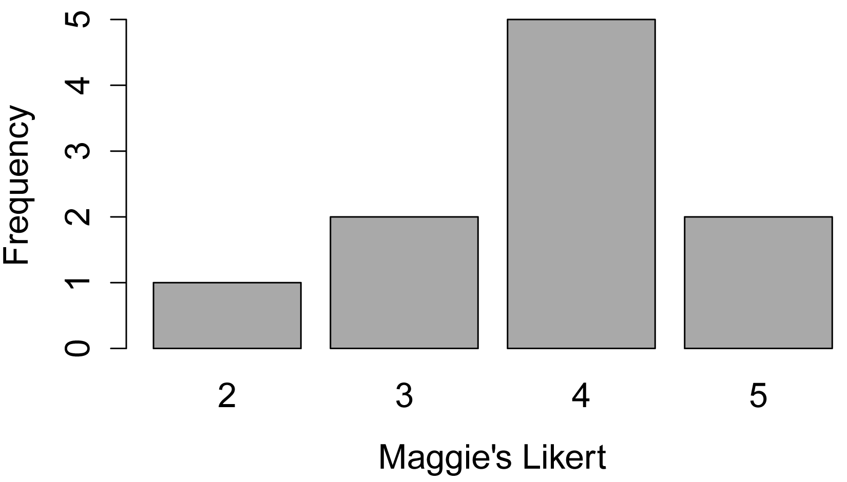
Bar plot

XT = xtabs(~ Likert.f,
          data=Data)

barplot(XT,
        col="dark gray",
        xlab="Maggie's Likert",
      ylab="Frequency")

Summarize data treating Likert scores as numeric

library(FSA)

Summarize(Likert ~ Speaker,
data=Data,
digits=3)

Speaker n mean sd min Q1 median Q3 max percZero
1 Maggie Simpson 10 3.8 0.919 2 3.25 4 4 5 0

One-sample Wilcoxon signed-rank test

wilcox.test function

In the wilcox.test function, the mu option indicates the value of the default value to compare to. In this example Data$Likert is the one-sample set of values on which to conduct the test. For the meaning of other options, see ?wilcox.test.

wilcox.test(Data$Likert,
            mu=3,
            conf.int=TRUE,
            conf.level=0.95)

Wilcoxon signed rank test with continuity correction

V = 32.5, p-value = 0.04007

alternative hypothesis: true location is not equal to 3

   ### Note p-value in the output above

   ### You will get the "cannot compute exact p-value with ties" error
   ###   You can ignore this, or use the exact=FALSE option.

95 percent confidence interval:
3.000044 4.500083

sample estimates:

(pseudo)median
      4.000032

   ### Note that the output will also produce a pseudo-median value
   ###   and a confidence interval if the conf.int=TRUE option is used.

wilcox.exact function

wilcox.exact(Data$Likert,
             mu=3,
             exact=TRUE,
             conf.int=TRUE,
             conf.level=0.95)

Exact Wilcoxon signed rank test

V = 32.5, p-value = 0.05469

alternative hypothesis: true mu is not equal to 3

95 percent confidence interval:

2 5

sample estimates:
(pseudo)median
3.75

Effect size

I am not aware of any established effect size statistic for the one-sample Wilcoxon signed-rank test. However, a version of the rank biserial correlation coefficient (rc) can be used. This is my recommendation. It is included for the matched pairs case in King, Rosopa, and Minimum (2000).

As an alternative, using a statistic analogous to the r used in the Mann–Whitney test may make sense.

The following interpretation is based on my personal intuition. It is not intended to be universal.

small

medium

Large

0.10 – < 0.30

0.30 – < 0.50

≥ 0.50

0.10 – < 0.40

0.40 – < 0.60

≥ 0.60

Rank biserial correlation coefficient

library(rcompanion)

wilcoxonOneSampleRC(Data$Likert, mu=3)

rc
0.806

library(rcompanion)

wilcoxonOneSampleRC(Data$Likert, mu=3, ci=TRUE)

rc lower.ci upper.ci

0.806 0.333 1

r

library(rcompanion)

wilcoxonOneSampleR(Data$Likert, mu=3)

r
0.674

wilcoxonOneSampleR(Data$Likert, mu=3, ci=TRUE)

r lower.ci upper.ci
0.674 0.2 0.914

References

King, B.M., P.J. Rosopa, E.W. and Minium. 2000. Statistical Reasoning in the Behavioral Sciences, 6^th. Wiley.

Exercises I

1. Considering Maggie Simpson’s data,

a. What was her median score?

b. What were the first and third quartiles for her scores?

c. According to the one-sample Wilcoxon signed-rank test, are her scores significantly different from a neutral score of 3?

d. Is the confidence interval output from the test useful in answering the previous question?

e. Overall, how would you summarize her results? Be sure to address the practical implication of her scores compared with a neutral score of 3.

f. Do these results reflect what you would expect from looking at the bar plot?

2. Brian Griffin wants to assess the education level of students in his course on creative writing for adults. He wants to know the median education level of his class, and if the education level of his class is different from the typical Bachelor’s level.

Brian used the following table to code his data.

Code   Abbreviation   Level

1      < HS           Less than high school
2        HS           High school
3        BA           Bachelor’s
4        MA           Master’s
5        PhD          Doctorate

The following are his course data.

Instructor       Student Education
'Brian Griffin' a        3
'Brian Griffin' b        2
'Brian Griffin' c        3
'Brian Griffin' d        3
'Brian Griffin' e        3
'Brian Griffin' f        3
'Brian Griffin' g        4
'Brian Griffin' h        5
'Brian Griffin' i        3
'Brian Griffin' j        4
'Brian Griffin' k        3
'Brian Griffin' l        2

For each of the following, answer the question, and show the output from the analyses you used to answer the question.

a. What was the median education level? (Be sure to report the education level, not just the numeric code!)

b. What were the first and third quartiles for education level?

b. According to the one-sample Wilcoxon signed-rank test, are the education levels significantly different from a typical level of Bachelor’s?

e. Is the confidence interval output from the test useful in answering the previous question?

f. Overall, how would you summarize the results? Be sure to address the practical implications.

g. Plot Brian’s data in a way that helps you visualize the data.

h. Do the results reflect what you would expect from looking at the plot?

Summary and Analysis of Extension Program Evaluation in R

One-sample Wilcoxon Signed-rank Test