![[banner]](images/banner.jpg "Cohansey River, Fairfield, New Jersey")
Median
For Likert item data, the primary measure of location we will use is the median. For a set of numbers, the median is the middle value when the data are arranged in numerical order. For example, for the set of values 1, 2, 3, 4, 5, 5, 5, the median value is 4. If there are an even number of values, the two middle values are averaged.
In concept, 50% of observations are less than the median, and 50% are greater than the median (ignoring the median itself in cases of an odd number of observations). You could also find the median of ordinal data consisting just of text descriptors. For example, for the set of values:
“high school”, “associate degree”, “bachelor’s degree”, “master’s degree”, “doctorate”,
the median is “bachelor’s degree”.
Using medians makes sense for ordinal data, whereas using means would in general not be appropriate.
Count of responses and bar plot
In order to visualize the location and variation of Likert item data, we will look at the distribution of the responses. The distribution of responses can be enumerated by counting the number of responses for each response level, and can be visualized with a bar plot of these counts. This is similar to a histogram of the responses.
Quartiles and percentiles
As a measure of the variation of data, it is also useful to look at the quartiles of the data set. The first quartile indicates the value below which 25% of the values fall. It is equivalent to the 25th percentile. The second quartile is equivalent to the median. The third quartile indicates the value below which 75% of the values fall. It is equivalent to the 75th percentile.
Packages used in this chapter
The packages used in this chapter include:
• psych
• FSA
• lattice
• ggplot2
• plyr
• boot
• rcompanion
The following commands will install these packages if they are not already installed:
if(!require(psych)){install.packages("psych")}
if(!require(FSA)){install.packages("FSA")}
if(!require(lattice)){install.packages("lattice")}
if(!require(ggplot2)){install.packages("ggplot2")}
if(!require(plyr)){install.packages("plyr")}
if(!require(boot)){install.packages("boot")}
if(!require(rcompanion)){install.packages("rcompanion")}
Descriptive statistics for one-sample data
Imagine a scenario in which 10 respondents are evaluating a single speaker on a single Likert item. The following example will create a data frame called Data consisting of three variables: Speaker, Rater, and Likert. The speaker is the same for all observations, and Likert represents the response on a five-point Likert item.
One-sample data
One-sample data refers to a single set of values that is not broken into groups. In this example, we have only one speaker with 10 ratings, hence one set of ratings values.
Variables and functions in this example
A new variable, Likert.f, will be created in the data frame. It will have the same values as the Likert variable, but we will tell R to treat it as an ordered factor variable, whereas Likert is a numeric variable. When summarizing data as a nominal variable, Likert.f will be used. But when summarizing data as a numeric variable, Likert will be used.
Note that the str function reports that Speaker is a factor variable, Rater and Likert are integer variables, and Likert.f is an ordered factor variable. The levels of the factor variables are shown with the level function.
Recall that Data$Likert tells R to use the Likert variable in the data frame Data.
Input =("
Speaker
Rater Likert
'Maggie Simpson' 1
3
'Maggie Simpson' 2
4
'Maggie Simpson' 3
5
'Maggie Simpson' 4
4
'Maggie Simpson' 5
4
'Maggie Simpson' 6
4
'Maggie Simpson' 7
4
'Maggie Simpson' 8
3
'Maggie Simpson' 9
2
'Maggie Simpson' 10
5
")
Data = read.table(textConnection(Input),header=TRUE)
### Create a new variable
which is the Likert scores as an ordered factor
Data$Likert.f
= factor(Data$Likert,
ordered = TRUE,
levels = c("1", "2", "3", "4", "5")
)
### Double check our
data frame
library(psych)
headTail(Data)
Speaker Rater Likert Likert.f
1 Maggie
Simpson 1 3
3
2 Maggie Simpson 2
4 4
3 Maggie
Simpson 3 5
5
4 Maggie Simpson 4
4 4
... <NA>
... ... <NA>
7
Maggie Simpson 7
4 4
8 Maggie
Simpson 8 3
3
9 Maggie Simpson 9
2 2
10 Maggie Simpson
10 5
5
str(Data)
'data.frame': 10 obs. of
4 variables:
$ Speaker : Factor w/ 1 level "Maggie Simpson":
1 1 1 1 1 1 1 1 1 1
$ Rater : int 1 2 3 4
5 6 7 8 9 10
$ Likert : int 3 4 5 4 4 4 4 3 2 5
$
Likert.f: Ord.factor w/ 5 levels "1"<"2"<"3"<"4"<..: 3 4
5 4 4 4 4 3 2 5
levels(Data$Speaker)
[1] "Maggie Simpson"
levels(Data$Likert.f)
[1] "1" "2" "3" "4" "5"
summary(Data)
### Remove unnecessary objects
rm(Input)
Summary treating Likert data as nominal data
The number of responses for each response level of Likert.f can be shown with the summary function, either on the Likert.f variable itself or as part of the whole data frame Data. The xtabs function can produce a similar summary.
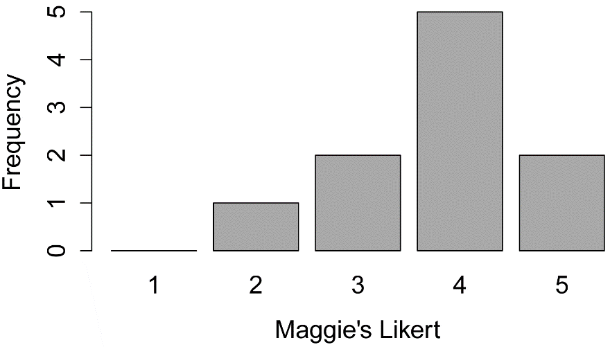
This same summary is then visualized with a bar plot.
summary(Data$Likert.f)
1 2 3 4 5
0 1 2 5 2
### The top row is the value
of Likert.f,
### and the next row is the counts
for each value.
summary(Data)
Speaker Rater
Likert Likert.f
Maggie Simpson:10
Min. : 1.00 Min. :2.00
1:0
1st Qu.: 3.25 1st Qu.:3.25 2:1
Median : 5.50 Median :4.00 3:2
Mean : 5.50 Mean :3.80
4:5
3rd Qu.: 7.75 3rd Qu.:4.00 5:2
Max. :10.00 Max. :5.00
xtabs and bar plot
XT = xtabs(~ Likert.f,
data=Data)
XT
Likert.f
1 2 3 4 5
0 1 2 5 2
### Counts for each level of Likert.f
sum(XT)
[1] 10
### Sum of counts for whole table
prop.table(XT)
1 2 3 4 5
0.0 0.1 0.2 0.5 0.2
### Proportion of total for each count
barplot(XT,
col="dark gray",
xlab="Maggie's Likert",
ylab="Frequency")
Summary treating Likert data as numeric data
In this code the Likert response data is treated as numeric data. The summary function produces the median, as well as the minimum, maximum, first quartile, and third quartile for a variable. The summary function can be used for either a single variable or a whole data frame. The Summarize function in the FSA package produces those statistics as well as the number of observations (n).
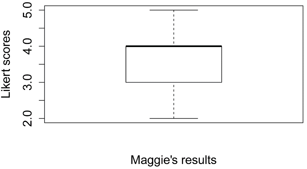
These statistics are visualized with a box plot. Note that the heavy line in the box is the median, and the ends of the box are the first quartile and third quartile. The extent of the whiskers in the box plot defaults to being the most extreme values, but no more than 1.5 times the length of the box itself. Values beyond the extent of the whiskers will be indicated with circles. Note that in the box plot for this example that the whiskers extend to the most extreme values in the data (2 and 5), and that there are no circles in the plot.
summary(Data$Likert)
Min. 1st Qu. Median
Mean 3rd Qu. Max.
2.00
3.25 4.00 3.80
4.00 5.00
summary(Data)
Speaker Rater
Likert Likert.f
Maggie Simpson:10
Min. : 1.00 Min. :2.00
1:0
1st Qu.: 3.25 1st Qu.:3.25 2:1
Median : 5.50 Median :4.00 3:2
Mean : 5.50 Mean :3.80
4:5
3rd Qu.: 7.75 3rd Qu.:4.00 5:2
Max. :10.00 Max. :5.00
library(FSA)
Summarize(Data$Likert,
digits=3)
n
mean sd
min Q1 median
Q3 max percZero
10.000
3.800 0.919 2.000
3.250 4.000 4.000
5.000 0.000
Box plot
boxplot(Data$Likert,
ylab="Likert scores",
xlab="Maggie's results")
Descriptive statistics for one-way or multi-way data
For this example, imagine that there are two speakers, each of which is being evaluated on each of three questions on 10-point Likert items. There are six raters, each of whom evaluates each speaker on each of these items.
One-way data
One-way data refers to a data set with a single measured variable but divided into groups. In this example looking at values of Likert for Spongebob and for Patrick would be an example of one-way data. Note that for one-way data there is a single dependent variable (Likert) and a single independent factor variable (Speaker).
Looking at Likert for the three levels of Question (Information, Presentation, and Questions) would also be an example of one-way data.
Multi-way data
Multi-way data refers to looking at a single measured variable divided into groups, where the groups are defined by at least two factor variables. If we look at values of Likert for each of the two speakers for each of the three questions, we are looking at two-way data.
Variables and functions in this example
The following example will create a data frame called Data consisting of four variables: Speaker, Question, Rater, and Likert. An additional variable named Likert.f will be created as an ordered factor variable with the same value as Likert for each observation.
Note that the str function reports that Speaker, Question, and Rater are factor variables, Likert is an integer variable, and Likert.f is an ordered factor variable. The levels of the factor variables are shown with the level function.
Recall that Data$Likert tells R to use the Likert variable in the data frame Data.
Input =("
Speaker
Question Rater Likert
Spongebob
Information a
5
Spongebob Information b
6
Spongebob Information
c 7
Spongebob Information
d 8
Spongebob Information
e 6
Spongebob Information
f 5
Spongebob Presentation
a 8
Spongebob Presentation
b 7
Spongebob Presentation
c 8
Spongebob Presentation
d 9
Spongebob Presentation
e 10
Spongebob Presentation
f 7
Spongebob Questions
a 3
Spongebob Questions
b 4
Spongebob Questions
c 5
Spongebob Questions
d 4
Spongebob Questions
e 6
Spongebob Questions
f 5
Patrick
Information a
6
Patrick Information
b 7
Patrick
Information c
8
Patrick Information
d 9
Patrick Information
e 7
Patrick
Information f
6
Patrick Presentation
a 9
Patrick
Presentation b 9
Patrick
Presentation c 10
Patrick
Presentation d 10
Patrick Presentation
e 8
Patrick
Presentation f 8
Patrick
Questions a
5
Patrick Questions
b 6
Patrick
Questions c
6
Patrick Questions
d 7
Patrick Questions e
5
Patrick Questions
f 7
")
Data = read.table(textConnection(Input),header=TRUE)
### Order factor levels,
otherwise R will alphabetize them
Data$Speaker = factor(Data$Speaker,
levels=unique(Data$Speaker))
Data$Question = factor(Data$Question,
levels=unique(Data$Question))
### Create an ordered factor of
Likert data
Data$Likert.f = factor(Data$Likert,
ordered=TRUE,
levels = c("1", "2", "3", "4", "5",
"6", "7", "8", "9", "10")
)
### Examine data frame
library(psych)
headTail(Data)
Speaker Question
Rater Likert Likert.f
1 Spongebob Information
a 5
5
2 Spongebob Information b
6 6
3 Spongebob
Information c
7 7
4 Spongebob
Information d
8 8
... <NA> <NA> <NA>
... <NA>
33 Patrick
Questions c 6
6
34 Patrick Questions
d 7
7
35 Patrick Questions
e 5
5
36 Patrick Questions
f 7
7
str(Data)
'data.frame': 36 obs. of
5 variables:
$ Speaker : Factor w/ 2 levels "Spongebob","Patrick":
1 1 1 1 1 1 1 1 1 1 ...
$ Question: Factor w/ 3 levels "Information",..:
1 1 1 1 1 1 2 2 2 2 ...
$ Rater : Factor w/ 6 levels
"a","b","c","d",..: 1 2 3 4 5 6 1 2 3 4 ...
$ Likert
: int 5 6 7 8 6 5 8 7 8 9 ...
$ Likert.f: Ord.factor
w/ 10 levels "1"<"2"<"3"<"4"<..: 5 6 7 8 6 5 8 7 8 9 ...
levels(Data$Speaker)
[1] "Spongebob" "Patrick"
levels(Data$Question)
[1] "Information" "Presentation" "Questions"
levels(Data$Rater)
[1] "a" "b" "c" "d" "e" "f"
levels(Data$Likert.f)
[1] "1" "2" "3" "4" "5"
"6" "7" "8" "9" "10"
summary(Data)
### Remove unnecessary objects
rm(Input)
Summary treating Likert data as nominal data
The number of responses for each response level of Likert.f
is shown with the summary function, but note that these counts are for
the entire data frame.
The xtabs function can be used to generate counts across groups. This
process is known as cross-tabulation, or cross-tabs. The
prop.table function, with the margin=1 option produces the proportions of
observations for each row.
This same summary is then visualized with a bar plot.
summary(Data)
Speaker Question Rater Likert Likert.f
Spongebob:18 Information :12 a:6 Min. : 3.000 6 :7
Patrick :18 Presentation:12 b:6 1st Qu.: 5.750 7 :7
Questions :12 c:6 Median : 7.000 5 :6
d:6 Mean : 6.833 8 :6
e:6 3rd Qu.: 8.000 9 :4
f:6 Max. :10.000 10 :3
(Other):3
XT = xtabs(~ Speaker + Likert.f, data=Data)
XT
Likert.f
Speaker 1 2 3 4 5 6 7 8 9 10
Spongebob 0 0 1 2 4 3 3 3 1 1
Patrick 0 0 0 0 2 4 4 3 3 2
prop.table(XT,
margin = 1)
Likert.f
Speaker 1 2 3 4 5 6 7 8 9 10
Spongebob 0.0000 0.0000 0.0556 0.1111 0.2222 0.1667 0.1667 0.1667 0.0556
0.0556
Patrick 0.0000 0.0000 0.0000 0.0000 0.1111 0.2222 0.2222 0.1667 0.1667 0.1111
sum(XT)
[1] 36
### Sum of counts in the table
rowSums(XT)
Spongebob Patrick
18 18
### Sum of counts for each row
colSums(XT)
1 2 3 4 5 6 7 8 9 10
0 0 1 2 6 7 7 6 4 3
### Sum of counts for each column
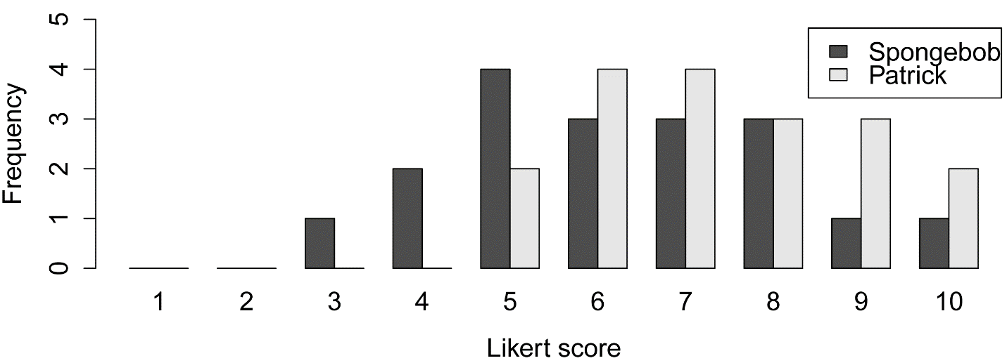
Bar plot by group
XT = xtabs(~ Speaker + Likert.f, data=Data)
XT
barplot(XT,
beside=TRUE,
legend=TRUE,
ylim=c(0, 5), # adjust to remove legend
overlap
xlab="Likert score",
ylab="Frequency")
xtabs to produce counts for two-way data
### Note that
the dependent variable (Likert.f)
### is the middle variable
in the formula
XT2 = xtabs(~ Speaker + Likert.f + Question,
data=Data)
XT2
, , Question = Information
Likert.f
Speaker 1 2 3 4 5 6 7 8 9 10
Spongebob 0 0 0 0 2 2 1 1 0 0
Patrick 0
0 0 0 0 2 2 1 1 0
, , Question = Presentation
Likert.f
Speaker 1 2 3 4 5 6 7 8 9 10
Spongebob 0 0 0 0 0 0 2 2 1 1
Patrick 0
0 0 0 0 0 0 2 2 2
, , Question = Questions
Likert.f
Speaker 1 2 3 4 5 6 7 8 9 10
Spongebob 0 0 1 2 2 1 0 0 0 0
Summary treating Likert data as numeric data
In this code the Likert response data is treated as numeric data. The summary function produces the median, quartiles, and extremes. But note that these statistics are for all values for the whole data frame.
The Summary function in the FSA package can produce these summary statistics across groups for one-way data or multi-way data.
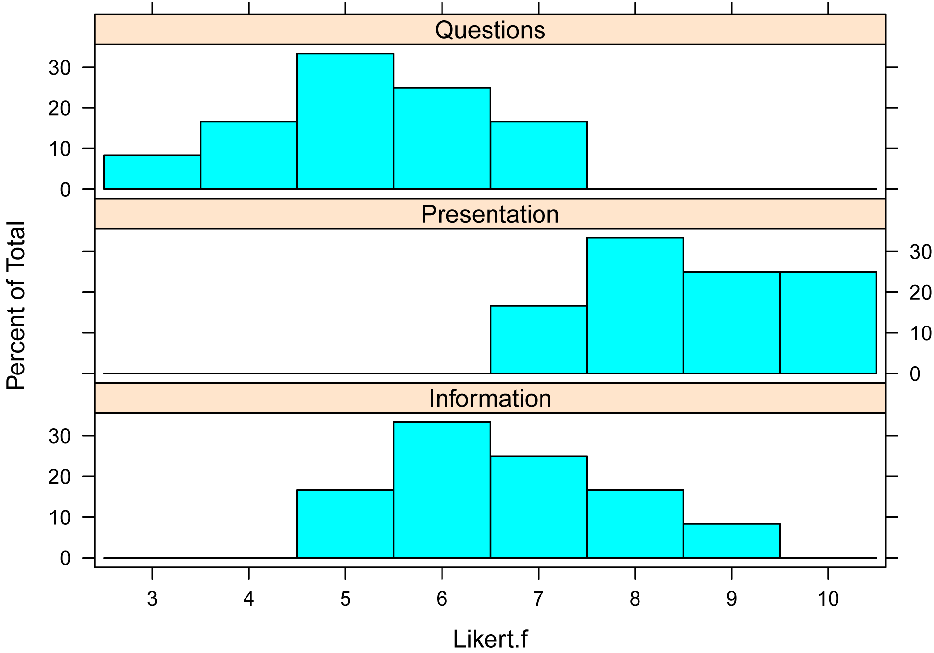
Histograms are then produced to visualize the distribution of responses across groups. Histograms for both one-way and two-way data can be produced with the histogram function in the lattice package.
Finally, box plots of the two-way data are produced.
summary(Data)
Speaker Question
Rater Likert
Likert.f
Spongebob:18 Information :12
a:6 Min. : 3.000 6
:7
Patrick :18 Presentation:12
b:6 1st Qu.: 5.750 7
:7
Questions :12 c:6 Median : 7.000
5 :6
d:6 Mean : 6.833 8
:6
e:6 3rd Qu.: 8.000 9
:4
f:6 Max. :10.000 10
:3
(Other):3
library(FSA)
Summarize(Likert ~ Question,
data=Data,
digits=3)
Question n
mean sd min Q1 median Q3 max
percZero
1 Information 12 6.667 1.231 5 6.00
6.5 7.25 9 0
2 Presentation 12 8.583 1.084 7 8.00 8.5
9.25 10 0
3
Questions 12 5.250 1.215 3 4.75 5.0 6.00
7 0
library(FSA)
Summarize(Likert ~ Speaker + Question,
data=Data,
digits=3)
Speaker
Question n mean sd min Q1 median
Q3 max percZero
1 Spongebob Information 6 6.167 1.169
5 5.25 6.0 6.75 8
0
2 Patrick Information 6 7.167 1.169
6 6.25 7.0 7.75 9
0
3 Spongebob Presentation 6 8.167 1.169 7 7.25
8.0 8.75 10 0
4
Patrick Presentation 6 9.000 0.894 8 8.25
9.0 9.75 10 0
5 Spongebob
Questions 6 4.500 1.049 3 4.00 4.5 5.00
6 0
6 Patrick
Questions 6 6.000 0.894 5 5.25 6.0 6.75
7 0
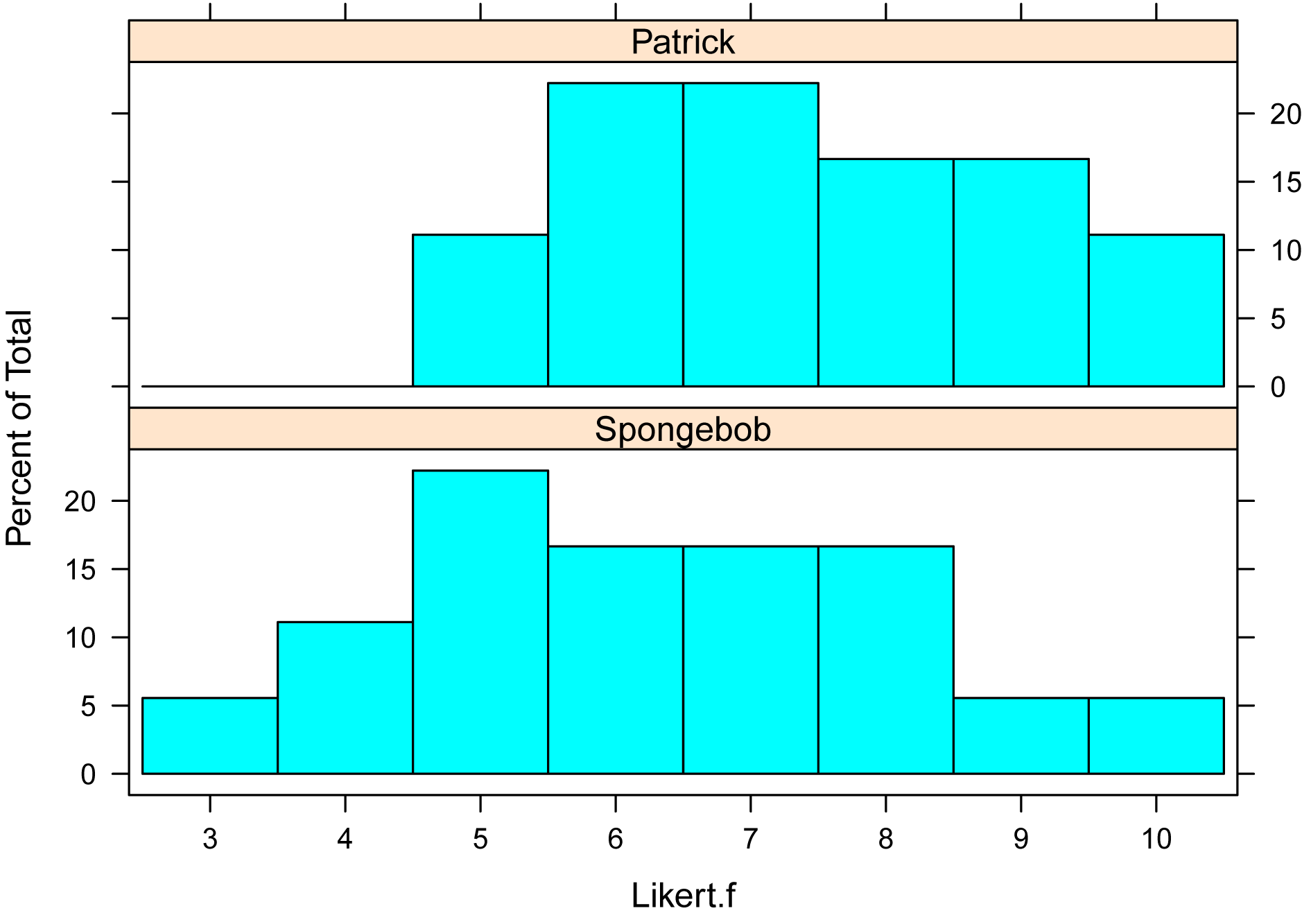
Bar plots by group
The histogram function in the lattice package will produce bar plots if the counted variable is ordinal in nature, as Likert.f is.
library(lattice)
histogram(~ Likert.f | Speaker,
data=Data,
layout=c(1,2)
# columns and rows of individual
plots
)
library(lattice)
histogram(~ Likert.f | Question,
data=Data,
layout=c(1,3)
# columns and rows of individual
plots
)
Bar plots for two-way data
library(lattice)
histogram(~ Likert.f | Speaker
+ Question,
data=Data,
layout=c(2,3)
# columns and rows of individual
plots
)

Box plots for two-way data
In general, using the names option is not necessary, but here it is useful because the default group names are long.
boxplot(Likert ~ Speaker + Question,
data=Data,
names=c("SB.Inf","P.Inf","SB.Pres",
"P.Pres", "SB.Quest", "P.Quest"),
ylab="Value")

### Note in this example,
SB is Spongebob, P is Patrick,
### Inf is
Information, Pres is Presentation,
###
and Quest is Question.
Interaction plot using medians and quartiles
Interaction plots are useful to visualize two-way data by plotting the value of a measured variable across the interaction of two factor variables.
In this example, the median Likert is calculated for each level of the interaction of two factors, and the first and third quartiles are used to indicate the spread of data about each median.
The Summarize function in the FSA package creates a data frame called Sum. The variables median, Q1, and Q3 in this data frame will then be used in the plot.
The interaction plot is produced with the ggplot2 package. This package is very versatile and powerful for creating plots, but the code can be intimidating at first. Note that the code indicates that the data frame to use is Sum, and the use of the variables Speaker, median, Question, Q1, Q3 from this data frame. Also note that the y axis label defined as “Median Likert score”.
### Create a
data frame called Sum with median and quartiles
library(FSA)
Sum = Summarize(Likert ~ Speaker + Question,
data=Data,
digits=3)
Sum
Speaker
Question n mean sd min Q1 median
Q3 max percZero
1 Spongebob Information 6 6.167 1.169
5 5.25 6.0 6.75 8
0
2 Patrick Information 6 7.167 1.169
6 6.25 7.0 7.75 9
0
3 Spongebob Presentation 6 8.167 1.169 7 7.25
8.0 8.75 10 0
4
Patrick Presentation 6 9.000 0.894 8 8.25
9.0 9.75 10 0
5 Spongebob
Questions 6 4.500 1.049 3 4.00 4.5 5.00
6 0
6 Patrick
Questions 6 6.000 0.894 5 5.25 6.0 6.75
7 0
### Produce interaction
plot
library(ggplot2)
pd = position_dodge(.2)
ggplot(Sum, aes(x=Speaker,
y=median,
color=Question)) +
geom_errorbar(aes(ymin=Q1,
ymax=Q3),
width=.2, size=0.7, position=pd) +
geom_point(shape=15,
size=4, position=pd) +
theme_bw() +
theme(axis.title = element_text(face = "bold")) +
ylab("Median Likert score")
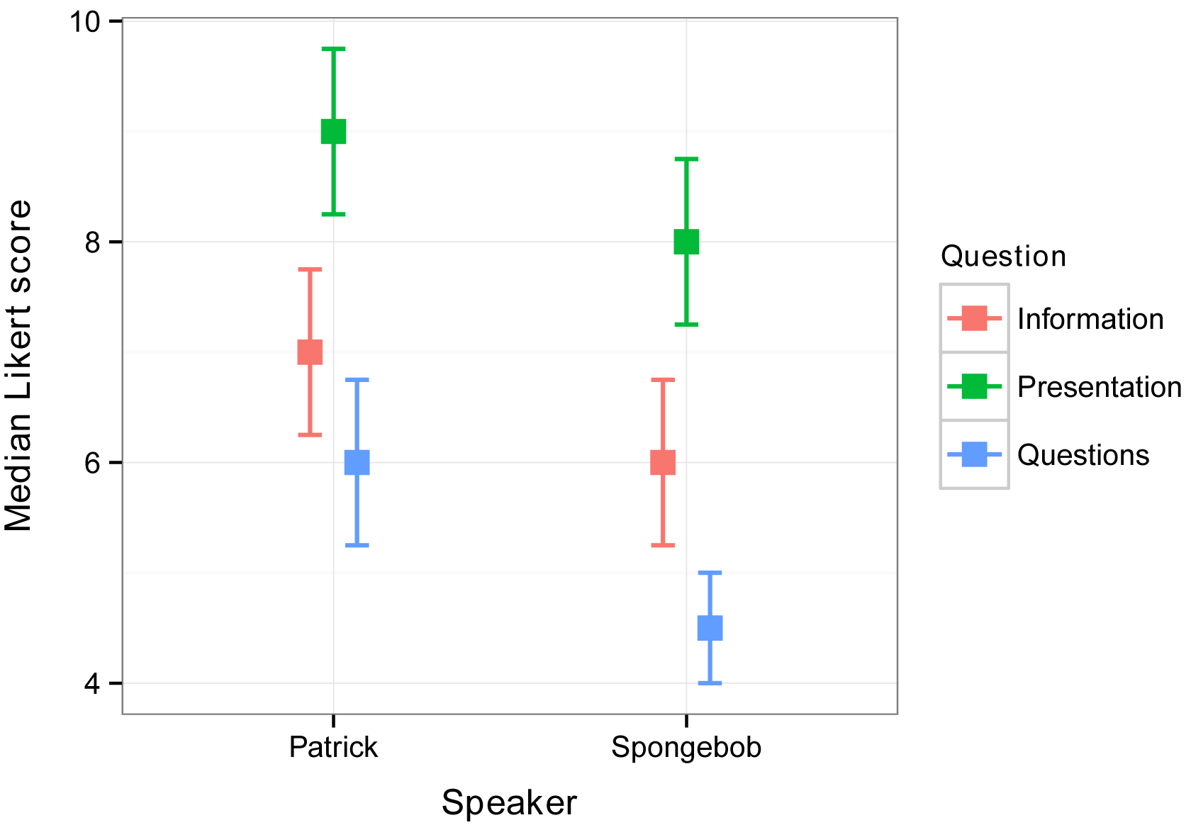
Interaction plot using medians and confidence intervals
An interaction plot can also use confidence intervals of the medians for its error bars. Confidence intervals are discussed in the Confidence Intervals chapter, and confidence intervals for medians are discussed in the Confidence Intervals for Medians chapter.
The function groupwiseMedian in the rcompanion package creates a data frame, called Sum, here that includes medians and confidence intervals of the medians for one-way or multi-way data. By default the function uses confidence intervals by the BCa method, but can produce confidence intervals by other methods. Note that bootstrapped confidence intervals may not be reliable for discreet data, such as the ordinal Likert data used in these examples, especially for small samples.
Also note that the order of speakers has changed from the previous interaction plot.
library(rcompanion)
Sum = groupwiseMedian(data = Data,
group
= c("Speaker", "Question"),
var
= "Likert",
conf=0.95,
R=5000)
Sum
Speaker
Question n Median Conf.level Bca.lower Bca.upper
1 Spongebob
Information 6 6.0
0.95 5
6.5
2 Spongebob Presentation 6 8.0
0.95 7
8.5
3 Spongebob Questions 6 4.5
0.95 3
5.0
4 Patrick Information 6 7.0
0.95 6
7.5
5 Patrick Presentation 6 9.0
0.95 8
9.5
6 Patrick Questions 6
6.0 0.95
5 6.5
Alternate code:
Sum = groupwiseMedian(data = Data,
group
= c("Speaker", "Question"),
var
= "Likert",
conf=0.95,
R=5000)
Sum
library(ggplot2)
pd = position_dodge(.2)
ggplot(Sum, aes(x=Speaker,
y=Median,
color=Question)) +
geom_errorbar(aes(ymin=Bca.lower,
ymax=Bca.upper),
width=.2, size=0.7, position=pd) +
geom_point(shape=15,
size=4, position=pd) +
theme_bw() +
theme(axis.title = element_text(face = "bold")) +
ylab("Median Likert score")

Descriptive statistics with opt-out responses
Opt-out responses include options like “don’t know” or “not applicable”. A typical approach to handling opt-out responses in Likert data is to separate them from the numeric or ordered factor responses of the question and report them separately.
For example, if responses to a question were 5, 5, 5, 4, 4, 2, ‘Don’t know’, ‘N/A’, you might report that you had 8 total responses, with 12.5% “Don’t know”, 12.5% “N/A”, and a median response of 4.5.
Analysis for vector data
The xtabs function can be used to count the levels of responses with opt-out answers, treating the data as nominal.
The Summarize function in the FSA will calculate the median for numeric data. Note that the numeric summary includes the number of observations and the number of “valid” observations, which excludes the non-numeric values.
Q1 = c("5", "5", "5", "4",
"4", "2", "Don't know", "N/A")
Counts of responses
Q1.f = as.factor(Q1)
XT = xtabs(~Q1)
XT
Q1
2 4 5 Don't know N/A
1 2 3 1 1
prop.table(XT)
Q1
2 4 5 Don't know N/A
0.125 0.250 0.375 0.125 0.125
Numerical summary of responses
Q1.n = as.numeric(Q1)
library(FSA)
Summarize(Q1.n,
digits = 2)
n nvalid mean sd min Q1 median Q3
max
8.00 6.00 4.17 1.17 2.00 4.00 4.50 5.00
5.00
Analysis for long-form data frame
Similar summaries can be obtained for data in a long-form
data frame.
Note that the read.table function by default reads in the values of Likert
as a factor variable, since it contains character values, not as a character
variable. Also note that you shouldn’t use NA for a value of “not
applicable” since NA is reserved by R for a missing value.
Input =("
Rater Question Likert
'1' Q1 5
'2' Q1 5
'3' Q1 5
'4' Q1 4
'5' Q1 4
'6' Q1 2
'7' Q1 DontKnow
'8' Q1 NotApp
'1' Q2 3
'2' Q2 3
'3' Q2 3
'4' Q2 2
'5' Q2 DontKnow
'6' Q2 2
'7' Q2 DontKnow
'8' Q2 DontKnow
'1' Q3 1
'2' Q3 2
'3' Q3 3
'4' Q3 2
'5' Q3 3
'6' Q3 1
'7' Q3 2
'8' Q3 3
")
Data = read.table(textConnection(Input),header=TRUE)
Counts of responses
XT = xtabs(~ Question + Likert,
data = Data)
XT
Likert
Question 1 2 3 4 5 DontKnow NotApp
Q1 0 1 0 2 3 1 1
Q2 0 2 3 0 0 3 0
Q3 2 3 3 0 0 0 0
### Counts for each question
prop.table(XT,
margin=1)
Likert
Question 1 2 3 4 5 DontKnow NotApp
Q1 0.000 0.125 0.000 0.250 0.375 0.125 0.125
Q2 0.000 0.250 0.375 0.000 0.000 0.375 0.000
Q3 0.250 0.375 0.375 0.000 0.000 0.000 0.000
### Proportions for each row
Numerical summary of responses
Data$Likert.n = as.numeric(as.character(Data$Likert))
library(FSA)
Summarize(Likert.n ~ Question,
data = Data)
Question n nvalid mean sd min Q1 median Q3 max percZero
1 Q1 8 6 4.166667 1.1690452 2 4.00 4.5 5 5 0
2 Q2 8 5 2.600000 0.5477226 2 2.00 3.0 3 3 0
3 Q3 8 8 2.125000 0.8345230 1 1.75 2.0 3 3 0
### Numerical summary
Summary for whole data frame
XT = xtabs( ~ Likert,
data = Data)
XT
Likert
1 2 3 4 5
DontKnow NotApp
2 6 6 2 3 4 1
prop.table(XT)
Likert
1 2 3 4 5 DontKnow NotApp
0.08333333 0.25000000 0.25000000 0.08333333 0.12500000 0.16666667 0.04166667
sum(XT)
[1] 24
### Sum of counts
in table
Summarize( ~
Likert.n,
data = Data,
digits = 2)
n nvalid mean sd min Q1 median
Q3 max
24.00 19.00 2.89 1.24 1.00 2.00 3.00 3.50
5.00
Exercises G
1. Considering Maggie Simpson's data,
a. How many Likert responses of "4" were there?
b. What percentage of responses was that?
c. What was the median Likert response?
d. What was the minimum response?
e. How would you summarize the bar plot of Maggie's responses?
2. Considering Spongebob and Patrick's workshops,
a. How many Likert responses of "5" did Spongebob
and Patrick get, respectively?
b. What percentage of total responses for each of them were
these?
c. How would you summarize the bar plot of their responses?
d. What were the median scores for Patrick for each of
Information, Presentation, and Questions?
e. What do the histograms for the two-way data (Spongebob and Patrick for each of Information, Presentation, and Questions) suggest to you?
f. Are your impressions borne out by the interaction plots?
g. Describe these results, including your opinions on the
practical implications.
3. Sandy Cheeks and Squidward each delivered presentations, and were each evaluated on each of the two courses (A and B).
Speaker Course Likert
Sandy A 5
Sandy A 5
Sandy A 5
Sandy A 4
Sandy A 3
Sandy A 3
Sandy B 5
Sandy B 4
Sandy B 3
Sandy B 3
Sandy B 2
Sandy B 2
Squidward A 4
Squidward A 4
Squidward A 3
Squidward A 3
Squidward A 2
Squidward A 2
Squidward B 3
Squidward B 3
Squidward B 2
Squidward B 2
Squidward B 1
Squidward B 1
a. Summarize the data as one-way or two-way data, using at least one plot, and at least one numerical summary. Interpret your results, and describe your conclusions. Remember to use statistics that are appropriate for Likert item data. Include your opinion on the practical importance.