![[banner]](images/banner.png "Batsto Lake, Wharton State Forest, New Jersey")
When to use it
The cricket example is shown in the “How to do the test” section.
Null hypotheses
Assumptions
How the test works
Examples
Graphing the results
Similar tests
See the Handbook for information on these topics.
How to do the test
Analysis of covariance example with two categories and type II sum of squares
This example uses type II sum of squares, but otherwise follows the example in the Handbook. The parameter estimates are calculated differently in R, so the calculation of the intercepts of the lines is slightly different.
###
--------------------------------------------------------------
### Analysis of covariance, cricket example
### pp. 228–229
### --------------------------------------------------------------
Input = ("
Species Temp Pulse
ex 20.8 67.9
ex 20.8 65.1
ex 24 77.3
ex 24 78.7
ex 24 79.4
ex 24 80.4
ex 26.2 85.8
ex 26.2 86.6
ex 26.2 87.5
ex 26.2 89.1
ex 28.4 98.6
ex 29 100.8
ex 30.4 99.3
ex 30.4 101.7
niv 17.2 44.3
niv 18.3 47.2
niv 18.3 47.6
niv 18.3 49.6
niv 18.9 50.3
niv 18.9 51.8
niv 20.4 60
niv 21 58.5
niv 21 58.9
niv 22.1 60.7
niv 23.5 69.8
niv 24.2 70.9
niv 25.9 76.2
niv 26.5 76.1
niv 26.5 77
niv 26.5 77.7
niv 28.6 84.7
")
Data = read.table(textConnection(Input),header=TRUE)
Simple plot
plot(x = Data$Temp,
y = Data$Pulse,
col = Data$Species,
pch = 16,
xlab = "Temperature",
ylab = "Pulse")
legend('bottomright',
legend = levels(Data$Species),
col = 1:2,
cex = 1,
pch = 16)
Analysis of covariance
options(contrasts = c("contr.treatment",
"contr.poly"))
### These are the default contrasts in R
model.1 = lm (Pulse ~ Temp + Species + Temp:Species,
data = Data)
library(car)
Anova(model.1, type="II")
Anova Table (Type II tests)
Sum Sq Df F value Pr(>F)
Temp 4376.1 1 1388.839 < 2.2e-16 ***
Species 598.0 1 189.789 9.907e-14 ***
Temp:Species 4.3 1 1.357 0.2542
### Interaction is not significant, so the slope across groups
### is not different.
model.2 = lm (Pulse ~ Temp + Species,
data = Data)
library(car)
Anova(model.2, type="II")
Anova Table (Type II tests)
Sum Sq Df F value Pr(>F)
Temp 4376.1 1 1371.4 < 2.2e-16 ***
Species 598.0 1 187.4 6.272e-14 ***
### The category variable (Species) is significant,
### so the intercepts among groups are different
summary(model.2)
Coefficients:
Estimate Std. Error t value Pr(>|t|)
(Intercept) -7.21091 2.55094 -2.827 0.00858 **
Temp 3.60275 0.09729 37.032 < 2e-16 ***
Speciesniv -10.06529 0.73526 -13.689 6.27e-14 ***
### Note that these estimates are different than in the Handbook,
### but the calculated results will be identical.
### The slope estimate is the same.
### The intercept for species 1 (ex) is (intercept).
### The intercept for species 2 (niv) is (intercept) + Speciesniv.
### This is determined from the contrast coding of the Species
### variable shown below, and the fact that Speciesniv is shown in
### coefficient table above.
contrasts(Data$Species)
niv
ex 0
niv 1
Simple plot with fitted lines
I.nought = -7.21091
I1 = I.nought + 0
I2 = I.nought + -10.06529
B = 3.60275
plot(x = Data$Temp,
y = Data$Pulse,
col = Data$Species,
pch = 16,
xlab = "Temperature",
ylab = "Pulse")
legend('bottomright',
legend = levels(Data$Species),
col = 1:2,
cex = 1,
pch = 16)
abline(I1, B,
lty=1, lwd=2, col = 1)
abline(I2, B,
lty=1, lwd=2, col = 2)

p-value and R-squared of combined model
summary(model.2)
Multiple R-squared: 0.9896, Adjusted R-squared: 0.9888
F-statistic: 1331 on 2 and 28 DF, p-value: < 2.2e-16
Checking assumptions of the model
hist(residuals(model.2),
col="darkgray")
A histogram of residuals from a linear model. The distribution of these residuals should be approximately normal.
plot(fitted(model.2),
residuals(model.2))

A plot of residuals vs. predicted values. The residuals should be unbiased and homoscedastic. For an illustration of these properties, see this diagram by Steve Jost at DePaul University: condor.depaul.edu/sjost/it223/documents/resid-plots.gif.
### additional model checking plots
with: plot(model.2)
### alternative: library(FSA);
residPlot(model.2)
# # #
Analysis of covariance example with three categories and type II sum of squares
This example uses type II sum of squares, and considers a case with three groups.
###
--------------------------------------------------------------
### Analysis of covariance, hypothetical data
### --------------------------------------------------------------
Input = ("
Species Temp Pulse
ex 20.8 67.9
ex 20.8 65.1
ex 24 77.3
ex 24 78.7
ex 24 79.4
ex 24 80.4
ex 26.2 85.8
ex 26.2 86.6
ex 26.2 87.5
ex 26.2 89.1
ex 28.4 98.6
ex 29 100.8
ex 30.4 99.3
ex 30.4 101.7
niv 17.2 44.3
niv 18.3 47.2
niv 18.3 47.6
niv 18.3 49.6
niv 18.9 50.3
niv 18.9 51.8
niv 20.4 60
niv 21 58.5
niv 21 58.9
niv 22.1 60.7
niv 23.5 69.8
niv 24.2 70.9
niv 25.9 76.2
niv 26.5 76.1
niv 26.5 77
niv 26.5 77.7
niv 28.6 84.7
fake 17.2 74.3
fake 18.3 77.2
fake 18.3 77.6
fake 18.3 79.6
fake 18.9 80.3
fake 18.9 81.8
fake 20.4 90
fake 21 88.5
fake 21 88.9
fake 22.1 90.7
fake 23.5 99.8
fake 24.2 100.9
fake 25.9 106.2
fake 26.5 106.1
fake 26.5 107
fake 26.5 107.7
fake 28.6 114.7
")
Data = read.table(textConnection(Input),header=TRUE)
Simple plot
plot(x = Data$Temp,
y = Data$Pulse,
col = Data$Species,
pch = 16,
xlab = "Temperature",
ylab = "Pulse")
legend('bottomright',
legend = levels(Data$Species),
col = 1:3,
cex = 1,
pch = 16)
Analysis of covariance
options(contrasts = c("contr.treatment",
"contr.poly"))
### These are the default contrasts in R
model.1 = lm (Pulse ~ Temp + Species + Temp:Species,
data = Data)
library(car)
Anova(model.1, type="II")
Sum Sq Df F value Pr(>F)
Temp 7026.0 1 2452.4187 <2e-16 ***
Species 7835.7 2 1367.5377 <2e-16 ***
Temp:Species 5.2 2 0.9126 0.4093
### Interaction is not significant, so the slope among groups
### is not different.
model.2 = lm (Pulse ~ Temp + Species,
data = Data)
library(car)
Anova(model.2, type="II")
Sum Sq Df F value Pr(>F)
Temp 7026.0 1 2462.2 < 2.2e-16 ***
Species 7835.7 2 1373.0 < 2.2e-16 ***
Residuals 125.6 44
### The category variable (Species) is significant,
### so the intercepts among groups are different
summary(model.2)
Coefficients:
Estimate Std. Error t value Pr(>|t|)
(Intercept) -6.35729 1.90713 -3.333 0.00175 **
Temp 3.56961 0.07194 49.621 < 2e-16 ***
Speciesfake 19.81429 0.66333 29.871 < 2e-16 ***
Speciesniv -10.18571 0.66333 -15.355 < 2e-16 ***
### The slope estimate is the Temp coefficient.
### The intercept for species 1 (ex) is (intercept).
### The intercept for species 2 (fake) is (intercept) + Speciesfake.
### The intercept for species 3 (niv) is (intercept) + Speciesniv.
### This is determined from the contrast coding of the Species
### variable shown below.
contrasts(Data$Species)
fake niv
ex 0 0
fake 1 0
niv 0 1
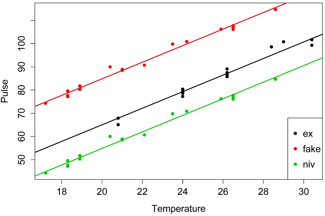
Simple plot with fitted lines
I.nought = -6.35729
I1 = I.nought + 0
I2 = I.nought + 19.81429
I3 = I.nought + -10.18571
B = 3.56961
plot(x = Data$Temp,
y = Data$Pulse,
col = Data$Species,
pch = 16,
xlab = "Temperature",
ylab = "Pulse")
legend('bottomright',
legend = levels(Data$Species),
col = 1:3,
cex = 1,
pch = 16)
abline(I1, B,
lty=1, lwd=2, col = 1)
abline(I2, B,
lty=1, lwd=2, col = 2)
abline(I3, B,
lty=1, lwd=2, col = 3)
p-value and R-squared of combined model
summary(model.2)
Multiple R-squared: 0.9919, Adjusted R-squared: 0.9913
F-statistic: 1791 on 3 and 44 DF, p-value: < 2.2e-16
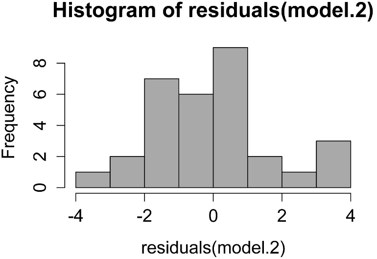
Checking assumptions of the model
hist(residuals(model.2),
col="darkgray")

A histogram of residuals from a linear model. The distribution of these residuals should be approximately normal.
plot(fitted(model.2),
residuals(model.2))

A plot of residuals vs. predicted values. The residuals should be unbiased and homoscedastic. For an illustration of these properties, see this diagram by Steve Jost at DePaul University: condor.depaul.edu/sjost/it223/documents/resid-plots.gif.
### additional model checking plots
with: plot(model.2)
### alternative: library(FSA);
residPlot(model.2)
# # #
Power analysis
See the Handbook for information on this topic.