An R Companion for the Handbook of Biological Statistics

Salvatore S. Mangiafico

Two-way Anova

Examples in Summary and Analysis of Extension Program Evaluation

SAEPER: Two-way ANOVA

SAEPER: Using Random Effects in Models
SAEPER: What are Least Square Means?

 

Packages used in this chapter

The following commands will install these packages if they are not already installed:

if(!require(FSA)){install.packages("FSA")}
if(!require(ggplot2)){install.packages("ggplot2")}
if(!require(car)){install.packages("car")}
if(!require(multcompView)){install.packages("multcompView")}
if(!require(lsmeans)){install.packages("lsmeans")}
if(!require(grid)){install.packages("grid")}
if(!require(nlme)){install.packages("nlme")}
if(!require(lme4)){install.packages("lme4")}
if(!require(lmerTest)){install.packages("lmerTest")} if(!require(rcompanion)){install.packages("rcompanion")}

 

When to use it

Null hypotheses

How the test works

Assumptions

See the Handbook for information on these topics.

 

Examples

The rattlesnake example is shown at the end of the “How to do the test” section.

 

How to do the test

For notes on linear models and conducting anova, see the “How to do the test” section in the One-way anova chapter of this book.  For two-way anova with robust regression, see the chapter on Two-way Anova with Robust Estimation.

 

Two-way anova example

 

### --------------------------------------------------------------
### Two-way anova, SAS example, pp. 179–180
### --------------------------------------------------------------

Input = ("
 id Sex     Genotype  Activity
  1 male    ff        1.884
  2 male    ff        2.283
  3 male    fs        2.396
  4 female  ff        2.838  
  5 male    fs        2.956
  6 female  ff        4.216
  7 female  ss        3.620
  8 female  ff        2.889  
  9 female  fs        3.550
 10 male    fs        3.105
 11 female  fs        4.556
 12 female  fs        3.087
 13 male    ff        4.939
 14 male    ff        3.486
 15 female  ss        3.079
 16 male    fs        2.649
 17 female  fs        1.943
 19 female  ff        4.198
 20 female  ff        2.473
 22 female  ff        2.033 
 24 female  fs        2.200
 25 female  fs        2.157
 26 male    ss        2.801
 28 male    ss        3.421
 29 female  ff        1.811
 30 female  fs        4.281
 32 female  fs        4.772
 34 female  ss        3.586
 36 female  ff        3.944
 38 female  ss        2.669
 39 female  ss        3.050
 41 male    ss        4.275 
 43 female  ss        2.963
 46 female  ss        3.236
 48 female  ss        3.673
 49 male    ss        3.110
")

Data = read.table(textConnection(Input),header=TRUE)

 

 

Means and summary statistics by group

 

library(Rmisc)

sum = summarySE(Data,
                measurevar="Activity",
                groupvars=c("Sex","Genotype"))
sum

 

     Sex Genotype N Activity        sd        se        ci

1 female       ff 8  3.05025 0.9599032 0.3393770 0.8024992

2 female       fs 8  3.31825 1.1445388 0.4046556 0.9568584

3 female       ss 8  3.23450 0.3617754 0.1279069 0.3024518

4   male       ff 4  3.14800 1.3745115 0.6872558 2.1871546

5   male       fs 4  2.77650 0.3168433 0.1584216 0.5041684

6   male       ss 4  3.40175 0.6348109 0.3174055 1.0101258

 

 

Interaction plot using summary statistics

 

library(ggplot2)

pd = position_dodge(.2)

ggplot(sum, aes(x=Genotype,
                y=Activity,
                color=Sex)) +
    geom_errorbar(aes(ymin=Activity-se,
                      ymax=Activity+se),
                   width=.2, size=0.7, position=pd) +
    geom_point(shape=15, size=4, position=pd) +
    theme_bw() +
    theme(
          axis.title.y = element_text(vjust= 1.8),
          axis.title.x = element_text(vjust= -0.5),
          axis.title = element_text(face = "bold")) +
    scale_color_manual(values = c("black", "blue"))

### You may see an error, “ymax not defined”
###  In this case, it does not appear to affect anything

 

 

Interaction plot for a two-way anova.  Square points represent means for groups, and error bars indicate standard errors of the mean.

 

 

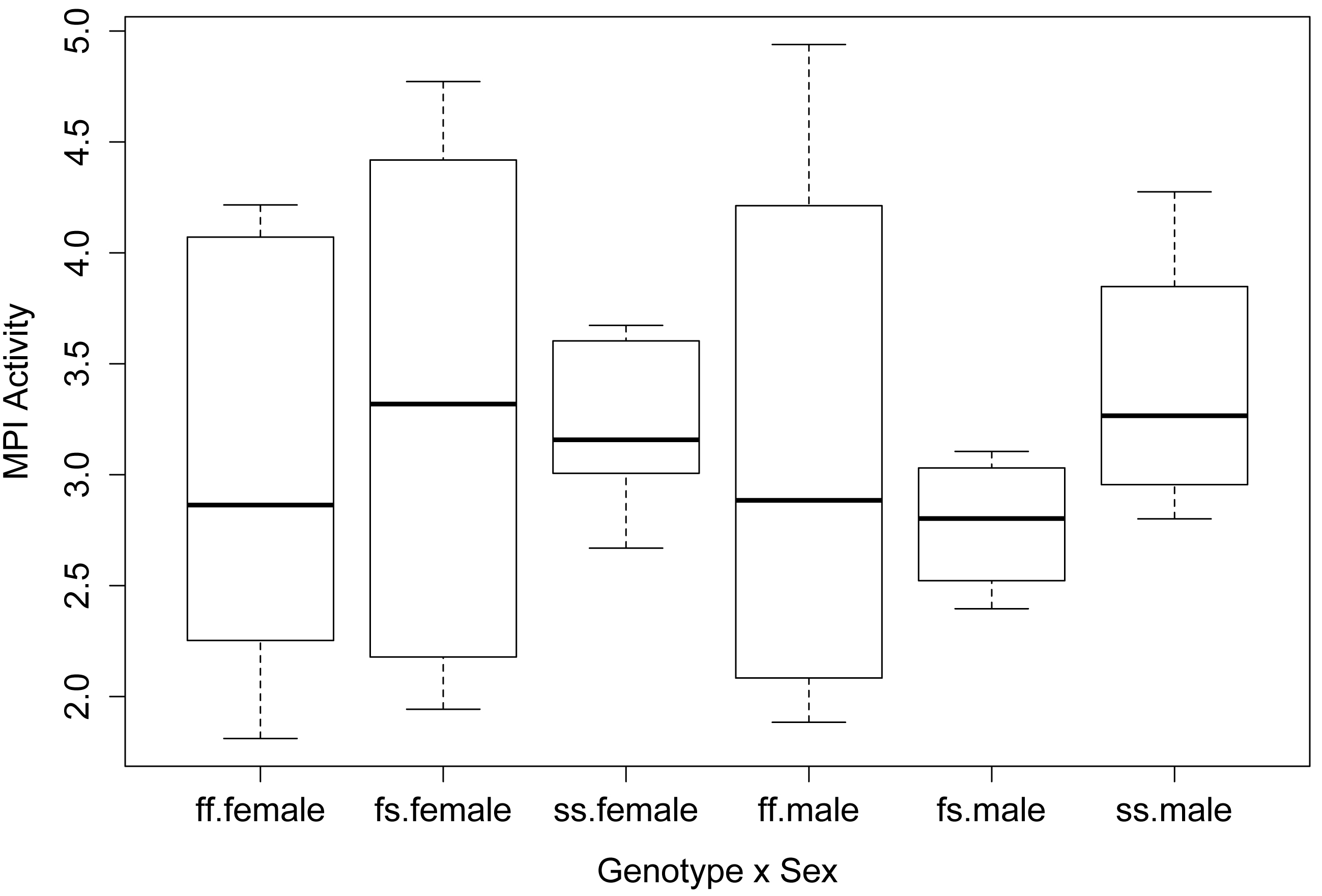
Simple box plot of main effect and interaction

 

boxplot(Activity ~ Genotype,
        data = Data,
        xlab = "Genotype",
        ylab = "MPI Activity")

 

 

 

boxplot(Activity ~ Genotype:Sex,
        data = Data,
        xlab = "Genotype x Sex",
        ylab = "MPI Activity")

 

 

Fit the linear model and conduct ANOVA

 

model = lm(Activity ~ Sex + Genotype + Sex:Genotype,
           data=Data)

library(car)

Anova(model, type="II")                    # Can use type="III"

   ### If you use type="III", you need the following line before the analysis
   ### options(contrasts = c("contr.sum", "contr.poly"))

 

              Sum Sq Df F value Pr(>F)

Sex           0.0681  1  0.0861 0.7712

Genotype      0.2772  2  0.1754 0.8400

Sex:Genotype  0.8146  2  0.5153 0.6025

Residuals    23.7138 30 

 

 

anova(model)                               # Produces type I sum of squares

 

             Df  Sum Sq Mean Sq F value Pr(>F)

Sex           1  0.0681 0.06808  0.0861 0.7712

Genotype      2  0.2772 0.13862  0.1754 0.8400

Sex:Genotype  2  0.8146 0.40732  0.5153 0.6025

Residuals    30 23.7138 0.79046

 

 

summary(model)     # Produces r-square, overall p-value, parameter estimates

 

Multiple R-squared:  0.04663, Adjusted R-squared:  -0.1123

F-statistic: 0.2935 on 5 and 30 DF,  p-value: 0.9128

 

 

Checking assumptions of the model

 

hist(residuals(model),
     col="darkgray")

 

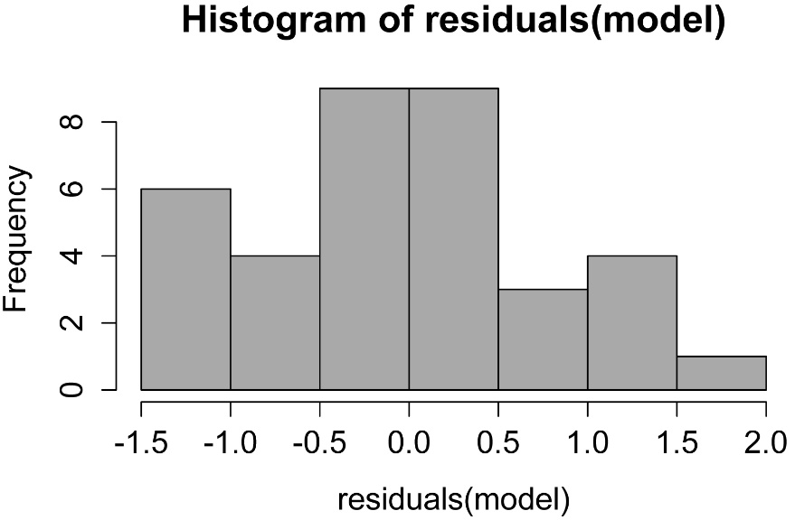
A histogram of residuals from a linear model.  The distribution of these residuals should be approximately normal.

 

 

plot(fitted(model),
     residuals(model))

 

 

A plot of residuals vs. predicted values.  The residuals should be unbiased and homoscedastic.  For an illustration of these properties, see this diagram by Steve Jost at DePaul University: condor.depaul.edu/sjost/it223/documents/resid-plots.gif.

 

 

### additional model checking plots with: plot(model)
### alternative: library(FSA); residPlot(model)

 

 

Post-hoc comparison of least-square means

For notes on least-square means, see the “Post-hoc comparison of least-square means” section in the Nested anova chapter in this book.

 

One advantage of the using the lsmeans package for post-hoc tests is that it can produce comparisons for interaction effects.

 

In general, if the interaction effect is significant, you will want to look at comparisons of means for the interactions.  If the interaction effect is not significant but a main effect is, it is appropriate to look at comparisons among the means for that main effect.  In this case, because no effect of Sex, Genotype, or Sex:Genotype was significant, we would not actually perform any mean separation test.

 

Mean separations for main factor with lsmeans

 

library(multcompView)
library(lsmeans)

lsmeans = lsmeans::lsmeans ### Uses the lsmeans function
                           ###  from the lsmeans package,
                           ###  not from the lmerTest package


leastsquare = lsmeans(model,
                      "Genotype",
                      adjust="tukey")

cld(leastsquare,
    alpha=.05,
    Letters=letters)

 

Genotype   lsmean        SE df lower.CL upper.CL .group

 fs       3.047375 0.2722236 30 2.359065 3.735685  a   

 ff       3.099125 0.2722236 30 2.410815 3.787435  a   

 ss       3.318125 0.2722236 30 2.629815 4.006435  a

 

    ### Means sharing a letter in .group are not significantly different

 

 

Mean separations for interaction effect with lsmeans

 

library(multcompView)
library(lsmeans)

lsmeans = lsmeans::lsmeans ### Uses the lsmeans function
                           ###  from the lsmeans package,
                           ###  not from the lmerTest package

leastsquare = lsmeans(model,
                      pairwise ~ Sex:Genotype,
                      adjust="tukey")

 

cld(leastsquare,
    alpha=.05, 
    Letters=letters)

    

Sex    Genotype  lsmean        SE df lower.CL upper.CL .group

 male   fs       2.77650 0.4445393 30 1.524666 4.028334  a   

 female ff       3.05025 0.3143368 30 2.165069 3.935431  a   

 male   ff       3.14800 0.4445393 30 1.896166 4.399834  a   

 female ss       3.23450 0.3143368 30 2.349319 4.119681  a   

 female fs       3.31825 0.3143368 30 2.433069 4.203431  a   

 male   ss       3.40175 0.4445393 30 2.149916 4.653584  a 

 

### Note that means are listed from low to high,

###  not in the same order as summarySE

 

 

Graphing the results

 

Simple bar plot with categories and no error bars

 

### Re-enter data as matrix

Input =("
Sex      ff       fs       ss
 Female  3.05025  3.31825  3.23450
 Male    3.14800  2.77650  3.40175
")

Matriz = as.matrix(read.table(textConnection(Input),
                   header=TRUE,
                   row.names=1))

Matriz

 

            ff      fs      ss

Female 3.05025 3.31825 3.23450

Male   3.14800 2.77650 3.40175

 

 

barplot(Matriz,
        beside=TRUE,
        legend=TRUE,
        ylim=c(0, 5),
        xlab="Genotype",
        ylab="MPI Activity")

 

 

Bar plot with error bars with ggplot2

This plot uses the data frame created by summarySE in Rmisc.  Error bars indicate standard error of the means (se in the data frame).

 

library(Rmisc)

sum = summarySE(Data, measurevar="Activity", groupvars=c("Sex","Genotype"))

sum

 

     Sex Genotype N Activity        sd        se        ci

1 female       ff 8  3.05025 0.9599032 0.3393770 0.8024992

2 female       fs 8  3.31825 1.1445388 0.4046556 0.9568584

3 female       ss 8  3.23450 0.3617754 0.1279069 0.3024518

4   male       ff 4  3.14800 1.3745115 0.6872558 2.1871546

5   male       fs 4  2.77650 0.3168433 0.1584216 0.5041684

6   male       ss 4  3.40175 0.6348109 0.3174055 1.0101258

 

 

### Plot adapted from:
###   shinyapps.stat.ubc.ca/r-graph-catalog/
 
library(ggplot2)
library(grid)

ggplot(sum,
   aes(x = Genotype, y = Activity, fill = Sex,
       ymax=Activity+se, ymin=Activity-se))  +
       geom_bar(stat="identity", position = "dodge", width = 0.7) +
       geom_bar(stat="identity", position = "dodge",
                colour = "black", width = 0.7,
                show_guide = FALSE)  +
       scale_y_continuous(breaks = seq(0, 4, 0.5),
                limits = c(0, 4),
                expand = c(0, 0))  +
       scale_fill_manual(name = "Count type" ,
                 values = c('grey80', 'grey30'),
                 labels = c("Female",
                            "Male"))  +
       geom_errorbar(position=position_dodge(width=0.7),
                     width=0.0, size=0.5, color="black")  +
       labs(x = "Genotype",
            y = "MPI Activity")  +
       ## ggtitle("Main title") +
       theme_bw()  +
       theme(panel.grid.major.x = element_blank(),
             panel.grid.major.y = element_line(colour = "grey50"),
             plot.title = element_text(size = rel(1.5),
             face = "bold", vjust = 1.5),
             axis.title = element_text(face = "bold"),
             legend.position = "top",
             legend.title = element_blank(),
             legend.key.size = unit(0.4, "cm"),
             legend.key = element_rect(fill = "black"),
             axis.title.y = element_text(vjust= 1.8),
             axis.title.x = element_text(vjust= -0.5)
           )

 

#     #     #

 

Bar plot for a two-way anova.  Bar heights represent means for groups, and error bars indicate standard errors of the mean.

 

 

Rattlesnake example – two-way anova without replication, repeated measures

This example could be interpreted as two-way anova without replication or as a one-way repeated measures experiment. Below it is analyzed as a two-way fixed effects model using the lm function, and as a mixed effects model using the nlme package and lme4 packages.

 

### --------------------------------------------------------------
### Two-way anova, rattlesnake example, pp. 177–178
### --------------------------------------------------------------

Input = ("
 Day  Snake  Openings
 1    D1        85
 1    D3       107
 1    D5        61
 1    D8        22
 1    D11       40
 1    D12       65
 2    D1        58
 2    D3        51
 2    D5        60
 2    D8        41
 2    D11       45
 2    D12       27
 3    D1        15
 3    D3        30
 3    D5        68
 3    D8        63
 3    D11       28
 3    D12        3
 4    D1        57
 4    D3        12
 4    D5        36
 4    D8        21
 4    D11       10
 4    D12       16
")

Data = read.table(textConnection(Input),header=TRUE)


### Treat Day as a factor variable

Data$Day = as.factor(Data$Day)

 

 

Using two-way fixed effects model

 

Means and summary statistics by group

 

library(Rmisc)

sum = summarySE(Data, measurevar="Openings", groupvars=c("Day"))

sum

 

  Day N Openings       sd        se       ci

1   1 6 63.33333 30.45434 12.432931 31.95987

2   2 6 47.00000 12.21475  4.986649 12.81859

3   3 6 34.50000 25.95958 10.597956 27.24291

4   4 6 25.33333 18.08498  7.383164 18.97903

 

 

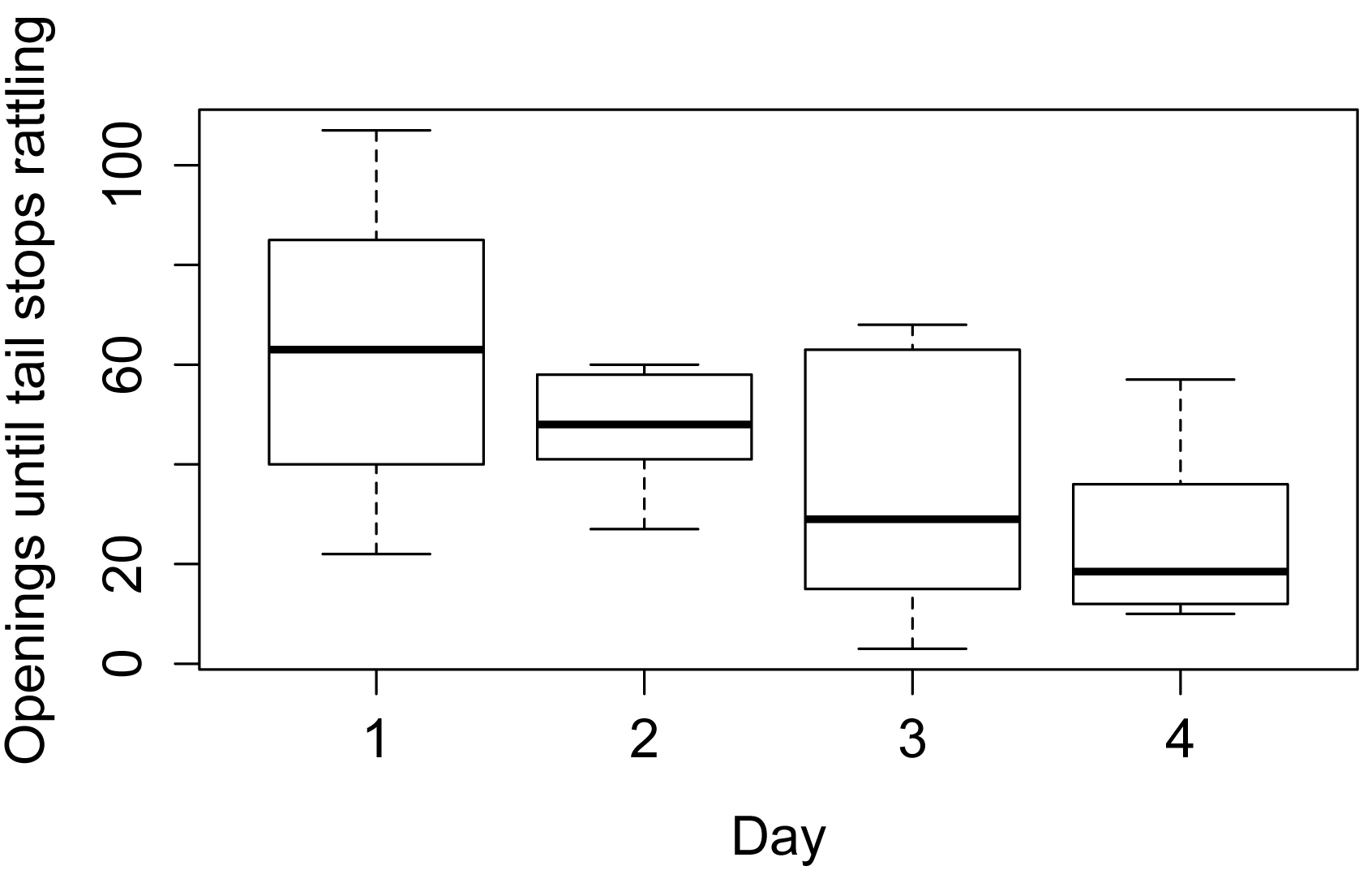
Simple box plots

 

boxplot(Openings ~ Day,
        data = Data,
        xlab = "Day",
        ylab = "Openings until tail stops rattling")

 

 

Fit the linear model and conduct ANOVA

 

model = lm(Openings ~ Day + Snake,
           data=Data)

library(car)

Anova(model, type="II")                    # Can use type="III"

 

          Sum Sq Df F value  Pr(>F) 

Day       4877.8  3  3.3201 0.04866 *

Snake     3042.2  5  1.2424 0.33818 

Residuals 7346.0 15                 

 

 

anova(model)                               # Produces type I sum of squares

 

          Df Sum Sq Mean Sq F value  Pr(>F) 

Day        3 4877.8 1625.93  3.3201 0.04866 *

Snake      5 3042.2  608.44  1.2424 0.33818 

Residuals 15 7346.0  489.73                 

 

 

summary(model)     # Produces r-square, overall p-value, parameter estimates

 

Multiple R-squared:  0.5188,  Adjusted R-squared:  0.2622

F-statistic: 2.022 on 8 and 15 DF,  p-value: 0.1142

 

 

Checking assumptions of the model

 

hist(residuals(model),
     col="darkgray")

 

A histogram of residuals from a linear model.  The distribution of these residuals should be approximately normal.

 

 

plot(fitted(model),
     residuals(model))

 

 

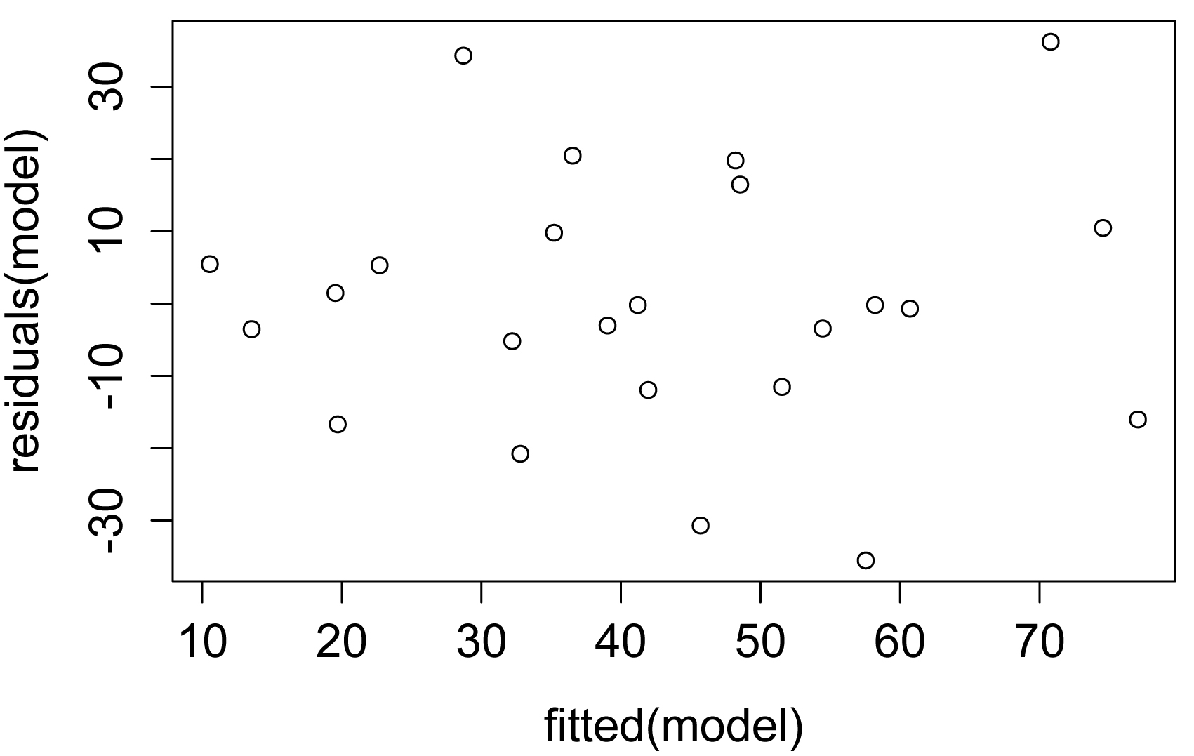
A plot of residuals vs. predicted values.  The residuals should be unbiased and homoscedastic.  For an illustration of these properties, see this diagram by Steve Jost at DePaul University: condor.depaul.edu/sjost/it223/documents/resid-plots.gif.

 

### additional model checking plots with: plot(model)
### alternative: library(FSA); residPlot(model)

 

 

Mean separations for main factor with lsmeans

 

For notes on least-square means, see the “Post-hoc comparison of least-square” means section in the Nested anova chapter in this book.  For other mean separation techniques for a main factor in anova, see “Tukey and Least Significant Difference mean separation tests (pairwise comparisons)” section in the One-way anova chapter.

 

library(multcompView)
library(lsmeans)

lsmeans = lsmeans::lsmeans ### Uses the lsmeans function
                           ###  from the lsmeans package,
                           ###  not from the lmerTest package

leastsquare = lsmeans(model,
                      "Day",
                      adjust="tukey")

cld(leastsquare,
    alpha=.05,
    Letters=letters)

 

Day   lsmean       SE df   lower.CL upper.CL .group

 4   25.33333 9.034476 15 -0.2085871 50.87525  a   

 3   34.50000 9.034476 15  8.9580796 60.04192  ab  

 2   47.00000 9.034476 15 21.4580796 72.54192  ab  

 1   63.33333 9.034476 15 37.7914129 88.87525   b 

 

    ### Means sharing a letter in .group are not significantly different

 

  

Using mixed effects model with nlme

This is an abbreviated example using the lme function in the nlme package.

library(nlme)

model = lme(Openings ~ Day, random=~1|Snake,
            data=Data,
            method="REML")

anova.lme(model,
          type="sequential",
          adjustSigma = FALSE)

            numDF denDF  F-value p-value
(Intercept)     1    15 71.38736  <.0001
Day             3    15  3.32005  0.0487

library(multcompView)
library(lsmeans)

lsmeans = lsmeans::lsmeans ### Uses the lsmeans function
                           ###  from the lsmeans package,
                           ###  not from the lmerTest package

leastsquare = lsmeans(model,
              "Day",
               adjust="tukey")

cld(leastsquare,
    alpha=.05,
    Letters=letters)

Day   lsmean       SE df asymp.LCL asymp.UCL .group
 4   25.33333 9.304196 NA  2.157372  48.50929  a   
 3   34.50000 9.304196 NA 11.324038  57.67596  ab  
 2   47.00000 9.304196 NA 23.824038  70.17596  ab  
 1   63.33333 9.304196 NA 40.157372  86.50929   b

   ### Means sharing a letter in .group are not significantly different

 

 

Using mixed effects model with lmer

This is an abbreviated example using the lmer function in the lme4 package.

library(lme4)
library(lmerTest)

model = lmer(Openings ~ Day + (1|Snake),
            data=Data,
            REML=TRUE)

anova(model)

Analysis of Variance Table of type III  with  Satterthwaite
approximation for degrees of freedom

    Sum Sq Mean Sq NumDF DenDF F.value  Pr(>F) 
Day 4877.8  1625.9     3    15  3.3201 0.04866 *

rand(model)

Analysis of Random effects Table:
      Chi.sq Chi.DF p.value
Snake 0.0915      1     0.8

Least square means with the lsmeans package

library(multcompView)
library(lsmeans)

lsmeans = lsmeans::lsmeans ### Uses the lsmeans function
                           ###  from the lsmeans package,
                           ###  not from the lmerTest package

leastsquare = lsmeans(model,
                     pairwise ~ Day,
                     alpha=.05,
                     adjust="tukey")

cld(leastsquare,
    alpha=.05, 
    Letters=letters,
    adjust="tukey")

Day   lsmean       SE    df   lower.CL upper.CL .group
 4   25.33333 9.304196 19.81 -0.1441779 50.81084  a   
 3   34.50000 9.304196 19.81  9.0224887 59.97751  ab  
 2   47.00000 9.304196 19.81 21.5224887 72.47751  ab  
 1   63.33333 9.304196 19.81 37.8558221 88.81084   b  

Degrees-of-freedom method: satterthwaite
Confidence level used: 0.95
Conf-level adjustment: sidak method for 4 estimates
P value adjustment: tukey method for comparing a family of 4 estimates
significance level used: alpha = 0.05

   ### Means sharing a letter in .group are not significantly different

Least square means using the lmerTest package

lsmeans = lmerTest::lsmeansLT ### Uses the lsmeans function
                              ###  from the lmerTest package,
                              ###  not from the lsmeans package

LT = lsmeans(model,
             test.effs = "Day")

LT

Least Squares Means table:
        Day Estimate Standard Error   DF t-value Lower CI Upper CI p-value   
Day  1  1.0    63.33           9.30 19.8    6.81    43.91     82.8  <2e-16 ***
Day  2  2.0    47.00           9.30 19.8    5.05    27.58     66.4   1e-04 ***
Day  3  3.0    34.50           9.30 19.8    3.71    15.08     53.9   0.001 **
Day  4  4.0    25.33           9.30 19.8    2.72     5.91     44.8   0.013 * 

PT = difflsmeans(model,
                 test.effs="Day")

PT

Differences of LSMEANS:

          Estimate Standard Error   DF t-value Lower CI Upper CI p-value  
Day 1 - 2     16.3          12.78 15.0    1.28   -10.90     43.6   0.220  
Day 1 - 3     28.8          12.78 15.0    2.26     1.60     56.1   0.039 *
Day 1 - 4     38.0          12.78 15.0    2.97    10.77     65.2   0.009 **
Day 2 - 3     12.5          12.78 15.0    0.98   -14.73     39.7   0.343  
Day 2 - 4     21.7          12.78 15.0    1.70    -5.57     48.9   0.111  
Day 3 - 4      9.2          12.78 15.0    0.72   -18.07     36.4   0.484  

### Extract lsmeans table

Sum = PT$diffs.lsmeans.table


### Extract comparisons and p-values

Comparison = rownames(Sum)

P.value   = Sum$'p-value'


### Adjust p-values

P.value.adj = p.adjust(P.value,
                       method =  "none")   

### Fix names of comparisons

Comparison = gsub("-", "- Day", Comparison)


### Produce compact letter display

library(rcompanion)

cldList(comparison = Comparison,
        p.value    = P.value.adj,
        threshold = 0.05)

  Group Letter MonoLetter
1  Day1      a         a
2  Day2     ab         ab
3  Day3      b          b
4  Day4      b          b

#     #     #

 

©2015 by Salvatore S. Mangiafico.
Rutgers Cooperative Extension, New Brunswick, NJ.

Organization of statistical tests and selection of examples for these tests ©2014 by John H. McDonald.  Used with permission.

Non-commercial reproduction of this content, with attribution, is permitted.  For-profit reproduction without permission is prohibited.

If you use the code or information in this site in a published work, please cite it as a source.  Also, if you are an instructor and use this book in your course, please let me know.   My contact information is on the About the Author page.

Citation:

Mangiafico, S.S. 2015. An R Companion for the Handbook of Biological Statistics, version 1.3.9, revised 2023.
rcompanion.org/rcompanion/. (Pdf version: rcompanion.org/documents/RCompanionBioStatistics.pdf.)