![[banner]](images/banner.png "Batsto Lake, Wharton State Forest, New Jersey")
Introduction
When to use it
Null hypothesis
How the test works
Assumptions
See the Handbook for information on these topics.
Example
Two-sample t-test, independent (unpaired) observations
### --------------------------------------------------------------
### Two-sample t-test, biological data analysis class, pp. 128–129
### --------------------------------------------------------------
Input =("
Group Value
2pm 69
2pm 70
2pm 66
2pm 63
2pm 68
2pm 70
2pm 69
2pm 67
2pm 62
2pm 63
2pm 76
2pm 59
2pm 62
2pm 62
2pm 75
2pm 62
2pm 72
2pm 63
5pm 68
5pm 62
5pm 67
5pm 68
5pm 69
5pm 67
5pm 61
5pm 59
5pm 62
5pm 61
5pm 69
5pm 66
5pm 62
5pm 62
5pm 61
5pm 70
")
Data = read.table(textConnection(Input),header=TRUE)
bartlett.test(Value ~ Group, data=Data)
### If p-value >= 0.05, use var.equal=TRUE below
Bartlett's K-squared = 1.2465, df = 1, p-value = 0.2642
t.test(Value ~ Group, data=Data,
var.equal=TRUE,
conf.level=0.95)
Two Sample t-test
t = 1.2888, df = 32, p-value = 0.2067
t.test(Value ~ Group, data=Data,
var.equal=FALSE,
conf.level=0.95)
Welch Two Sample t-test
t = 1.3109, df = 31.175, p-value = 0.1995
Plot of histograms
library(lattice)
histogram(~ Value | Group,
data=Data,
layout=c(1,2) # columns and rows of
individual plots
)
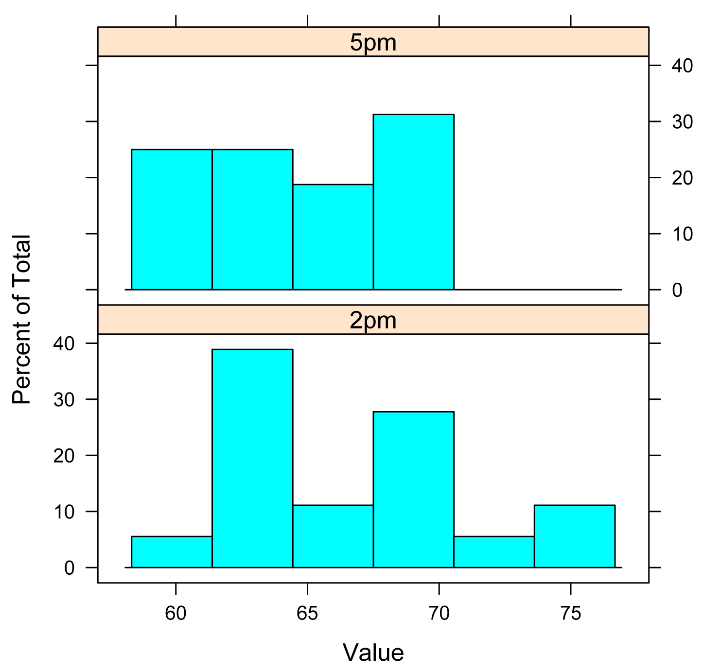
Histograms for each population in a two-sample t-test. For the t-test to be valid, the data in each population should be approximately normal. If the distributions are different, minimally Welch’s t-test should be used. If the data are not normal or the distributions are different, a non-parametric test like Mann-Whitney U-test or permutation test may be appropriate.
Box plots
boxplot(Value ~ Group,
data = Data,
names=c("2 pm","5 pm"),
ylab="Value")
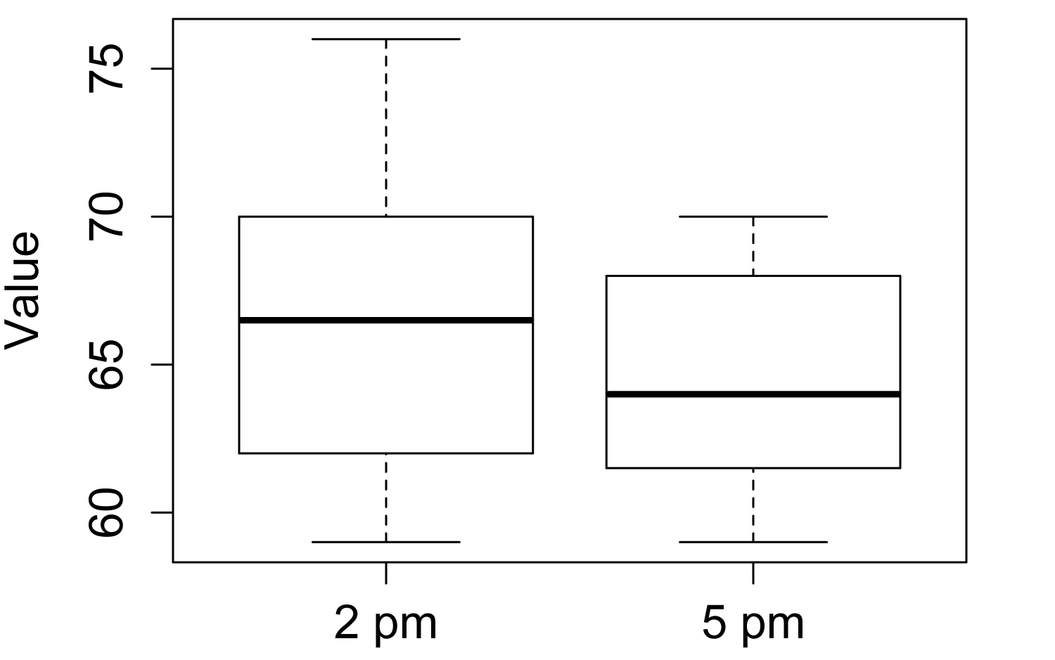
Box plots of two populations from a two-sample t-test.
# # #
Similar tests
Welch’s t-test is discussed below. The
paired t-test and signed-rank test are discussed in
this book in their own chapters. Analysis of variance (anova)
is discussed in several subsequent chapters.
As non-parametric
alternatives, the Mann–Whitney U-test and the permutation
test for two independent samples are discussed in the chapter
Mann–Whitney and Two-sample Permutation Test.
Welch’s t-test
Welch’s t-test is shown above in the “Example” section (“Two sample unpaired t-test”). It is invoked with the var.equal=FALSE option in the t.test function.
How to do the test
The SAS example from the Handbook is shown above in the “Example” section.
Power analysis
Power analysis for t-test
###
--------------------------------------------------------------
### Power analysis, t-test, wide feet, p. 131
### --------------------------------------------------------------
M1 = 100.6 # Mean for sample
1
M2 = 103.6 # Mean for sample 2
S1 = 5.26 # Std dev for
sample 1
S2 = 5.26 # Std dev for
sample 2
Cohen.d = (M1 - M2)/sqrt(((S1^2) + (S2^2))/2)
library(pwr)
pwr.t.test(
n = NULL, # Observations in
_each_ group
d = Cohen.d,
sig.level = 0.05, # Type I
probability
power = 0.90, # 1 minus Type II
probability
type = "two.sample", #
Change for one- or two-sample
alternative = "two.sided")
Two-sample t test power calculation
n = 65.57875 # Number for each group
# # #