![[banner]](images/banner.png "Batsto Lake, Wharton State Forest, New Jersey")
When to use it
The bird example is shown in the “How to do multiple logistic regression” section.
Null hypothesis
How it works
Selecting variables in multiple logistic regression
See the Handbook for information on these topics.
Assumptions
See the Handbook and the “How to do multiple logistic regression” section below for information on this topic.
Example
Graphing the results
Similar tests
See the Handbook for information on these topics.
Packages used in this chapter
The following commands will install these packages if they are not already installed:
if(!require(dplyr)){install.packages("dplyr")}
if(!require(FSA){install.packages("FSA")}
if(!require(psych)){install.packages("psych")}
if(!require(rcompanion)){install.packages("rcompanion")}
if(!require(car){install.packages("car")}
if(!require(lmtest)){install.packages("lmtest")}
if(!require(PerformanceAnalytics)){install.packages("PerformanceAnalytics")}
How to do multiple logistic regression
Don’t use stepwise procedures
In general, stepwise procedures are not recommended to determine an appropriate model for multiple regression. It is better to use knowledge of the measured variables, or to use penalized models like ridge regression or lasso regression.
However, a stepwise procedure will be used here to highlight some methods to compare models, and to compare with the example in the Handbook.
Stepwise regression in R
Multiple logistic regression can be determined by a stepwise procedure using the step function. This function selects models to minimize AIC, not according to p-values as does the SAS example in the Handbook. Note, also, that in this example the step function found a different model than did the procedure in the Handbook.
It is often advised to not blindly follow a stepwise procedure, but to also compare competing models using fit statistics (AIC, AICc, BIC), or to build a model from available variables that are biologically or scientifically sensible.
Multiple correlation
Multiple correlation is one tool for investigating the relationship among potential independent variables. For example, if two independent variables are correlated to one another, likely both won’t be needed in a final model, but there may be reasons why you would choose one variable over the other.
###
--------------------------------------------------------------
### Multiple logistic regression, bird example, p. 254–256
### --------------------------------------------------------------
### When using read.table, the column headings need to be on the
### same line. If the headings will spill over to the next line,
### be sure to not put an enter or return at the end of the top
### line. The same holds for each line of data.
Data = read.table(header=TRUE, stringsAsFactors=TRUE, text="
Species Status Length Mass Range Migr Insect Diet Clutch Broods Wood Upland
Water Release Indiv
Cyg_olor 1 1520 9600 1.21 1 12 2 6 1 0 0 1
6 29
Cyg_atra 1 1250 5000 0.56 1 0 1 6 1 0 0 1
10 85
Cer_nova 1 870 3360 0.07 1 0 1 4 1 0 0 1
3 8
Ans_caer 0 720 2517 1.1 3 12 2 3.8 1 0 0 1
1 10
Ans_anse 0 820 3170 3.45 3 0 1 5.9 1 0 0 1
2 7
Bra_cana 1 770 4390 2.96 2 0 1 5.9 1 0 0 1
10 60
Bra_sand 0 50 1930 0.01 1 0 1 4 2 0 0 0
1 2
Alo_aegy 0 680 2040 2.71 1 NA 2 8.5 1 0 0 1
1 8
Ana_plat 1 570 1020 9.01 2 6 2 12.6 1 0 0 1
17 1539
Ana_acut 0 580 910 7.9 3 6 2 8.3 1 0 0 1
3 102
Ana_pene 0 480 590 4.33 3 0 1 8.7 1 0 0 1
5 32
Aix_spon 0 470 539 1.04 3 12 2 13.5 2 1 0 1
5 10
Ayt_feri 0 450 940 2.17 3 12 2 9.5 1 0 0 1
3 9
Ayt_fuli 0 435 684 4.81 3 12 2 10.1 1 0 0 1
2 5
Ore_pict 0 275 230 0.31 1 3 1 9.5 1 1 1 0
9 398
Lop_cali 1 256 162 0.24 1 3 1 14.2 2 0 0 0
15 1420
Col_virg 1 230 170 0.77 1 3 1 13.7 1 0 0 0
17 1156
Ale_grae 1 330 501 2.23 1 3 1 15.5 1 0 1 0
15 362
Ale_rufa 0 330 439 0.22 1 3 2 11.2 2 0 0 0
2 20
Per_perd 0 300 386 2.4 1 3 1 14.6 1 0 1 0
24 676
Cot_pect 0 182 95 0.33 3 NA 2 7.5 1 0 0 0
3 NA
Cot_aust 1 180 95 0.69 2 12 2 11 1 0 0 1
11 601
Lop_nyct 0 800 1150 0.28 1 12 2 5 1 1 1 0
4 6
Pha_colc 1 710 850 1.25 1 12 2 11.8 1 1 0 0
27 244
Syr_reev 0 750 949 0.2 1 12 2 9.5 1 1 1 0
2 9
Tet_tetr 0 470 900 4.17 1 3 1 7.9 1 1 1 0
2 13
Lag_lago 0 390 517 7.29 1 0 1 7.5 1 1 1 0
2 4
Ped_phas 0 440 815 1.83 1 3 1 12.3 1 1 0 0
1 22
Tym_cupi 0 435 770 0.26 1 4 1 12 1 0 0 0
3 57
Van_vane 0 300 226 3.93 2 12 3 3.8 1 0 0 0
8 124
Plu_squa 0 285 318 1.67 3 12 3 4 1 0 0 1
2 3
Pte_alch 0 350 225 1.21 2 0 1 2.5 2 0 0 0
1 8
Pha_chal 0 320 350 0.6 1 12 2 2 2 1 0 0
8 42
Ocy_loph 0 330 205 0.76 1 0 1 2 7 1 0 1
4 23
Leu_mela 0 372 NA 0.07 1 12 2 2 1 1 0 0
6 34
Ath_noct 1 220 176 4.84 1 12 3 3.6 1 1 0 0
7 221
Tyt_alba 0 340 298 8.9 2 0 3 5.7 2 1 0 0
1 7
Dac_nova 1 460 382 0.34 1 12 3 2 1 1 0 0
7 21
Lul_arbo 0 150 32.1 1.78 2 4 2 3.9 2 1 0 0
1 5
Ala_arve 1 185 38.9 5.19 2 12 2 3.7 3 0 0 0
11 391
Pru_modu 1 145 20.5 1.95 2 12 2 3.4 2 1 0 0
14 245
Eri_rebe 0 140 15.8 2.31 2 12 2 5 2 1 0 0
11 123
Lus_mega 0 161 19.4 1.88 3 12 2 4.7 2 1 0 0
4 7
Tur_meru 1 255 82.6 3.3 2 12 2 3.8 3 1 0 0
16 596
Tur_phil 1 230 67.3 4.84 2 12 2 4.7 2 1 0 0
12 343
Syl_comm 0 140 12.8 3.39 3 12 2 4.6 2 1 0 0
1 2
Syl_atri 0 142 17.5 2.43 2 5 2 4.6 1 1 0 0
1 5
Man_mela 0 180 NA 0.04 1 12 3 1.9 5 1 0 0
1 2
Man_mela 0 265 59 0.25 1 12 2 2.6 NA 1 0 0
1 80
Gra_cyan 0 275 128 0.83 1 12 3 3 2 1 0 1
1 NA
Gym_tibi 1 400 380 0.82 1 12 3 4 1 1 0 0
15 448
Cor_mone 0 335 203 3.4 2 12 2 4.5 1 1 0 0
2 3
Cor_frug 1 400 425 3.73 1 12 2 3.6 1 1 0 0
10 182
Stu_vulg 1 222 79.8 3.33 2 6 2 4.8 2 1 0 0
14 653
Acr_tris 1 230 111.3 0.56 1 12 2 3.7 1 1 0 0
5 88
Pas_dome 1 149 28.8 6.5 1 6 2 3.9 3 1 0 0
12 416
Pas_mont 0 133 22 6.8 1 6 2 4.7 3 1 0 0
3 14
Aeg_temp 0 120 NA 0.17 1 6 2 4.7 3 1 0 0
3 14
Emb_gutt 0 120 19 0.15 1 4 1 5 3 0 0 0
4 112
Poe_gutt 0 100 12.4 0.75 1 4 1 4.7 3 0 0 0
1 12
Lon_punc 0 110 13.5 1.06 1 0 1 5 3 0 0 0
1 8
Lon_cast 0 100 NA 0.13 1 4 1 5 NA 0 0 1
4 45
Pad_oryz 0 160 NA 0.09 1 0 1 5 NA 0 0 0
2 6
Fri_coel 1 160 23.5 2.61 2 12 2 4.9 2 1 0 0
17 449
Fri_mont 0 146 21.4 3.09 3 10 2 6 NA 1 0 0
7 121
Car_chlo 1 147 29 2.09 2 7 2 4.8 2 1 0 0
6 65
Car_spin 0 117 12 2.09 3 3 1 4 2 1 0 0
3 54
Car_card 1 120 15.5 2.85 2 4 1 4.4 3 1 0 0
14 626
Aca_flam 1 115 11.5 5.54 2 6 1 5 2 1 0 0
10 607
Aca_flavi 0 133 17 1.67 2 0 1 5 3 0 1 0
3 61
Aca_cann 0 136 18.5 2.52 2 6 1 4.7 2 1 0 0
12 209
Pyr_pyrr 0 142 23.5 3.57 1 4 1 4 3 1 0 0
2 NA
Emb_citr 1 160 28.2 4.11 2 8 2 3.3 3 1 0 0
14 656
Emb_hort 0 163 21.6 2.75 3 12 2 5 1 0 0 0
1 6
Emb_cirl 1 160 23.6 0.62 1 12 2 3.5 2 1 0 0
3 29
Emb_scho 0 150 20.7 5.42 1 12 2 5.1 2 0 0 1
2 9
Pir_rubr 0 170 31 0.55 3 12 2 4 NA 1 0 0
1 2
Age_phoe 0 210 36.9 2 2 8 2 3.7 1 0 0 1
1 2
Stu_negl 0 225 106.5 1.2 2 12 2 4.8 2 0 0 0
1 2
")
Create a data frame of numeric variables
### Select only those variables that
are numeric or can be made numeric
library(dplyr)
Data.num =
select(Data,
Status,
Length,
Mass,
Range,
Migr,
Insect,
Diet,
Clutch,
Broods,
Wood,
Upland,
Water,
Release,
Indiv)
### Covert integer variables to numeric variables
Data.num$Status = as.numeric(Data.num$Status)
Data.num$Length = as.numeric(Data.num$Length)
Data.num$Migr = as.numeric(Data.num$Migr)
Data.num$Insect = as.numeric(Data.num$Insect)
Data.num$Diet = as.numeric(Data.num$Diet)
Data.num$Broods = as.numeric(Data.num$Broods)
Data.num$Wood = as.numeric(Data.num$Wood)
Data.num$Upland = as.numeric(Data.num$Upland)
Data.num$Water = as.numeric(Data.num$Water)
Data.num$Release = as.numeric(Data.num$Release)
Data.num$Indiv = as.numeric(Data.num$Indiv)
### Examine the new data frame
library(FSA)
headtail(Data.num)
Status Length Mass Range Migr Insect Diet Clutch Broods Wood Upland Water Release Indiv
1 1 1520 9600.0 1.21 1 12 2 6.0 1 0 0 1 6 29
2 1 1250 5000.0 0.56 1 0 1 6.0 1 0 0 1 10 85
3 1 870 3360.0 0.07 1 0 1 4.0 1 0 0 1 3 8
77 0 170 31.0 0.55 3 12 2 4.0 NA 1 0 0 1 2
78 0 210 36.9 2.00 2 8 2 3.7 1 0 0 1 1 2
79 0 225 106.5 1.20 2 12 2 4.8 2 0 0 0 1 2
Examining correlations among variables
### Note I used Spearman correlations
here
library(PerformanceAnalytics)
chart.Correlation(Data.num,
method="spearman",
histogram=TRUE,
pch=16)

library(psych)
corr.test(Data.num,
use = "pairwise",
method="spearman",
adjust="none", # Can
adjust p-values; see ?p.adjust for options
alpha=.05)
Multiple logistic regression example
In this example, the data contain missing values. In SAS, missing values are indicated with a period, whereas in R missing values are indicated with NA. SAS will often deal with missing values seamlessly. While this makes things easier for the user, it may not ensure that the user understands what is being done with these missing values. In some cases, R requires that user be explicit with how missing values are handled.
One method to handle missing values in a multiple regression would be to remove all observations from the data set that have any missing values. This is what we will do prior to the stepwise procedure, creating a data frame called Data.omit.
However, when we create our final model, we may want to exclude only those observations that have missing values in the variables that are actually included in that final model.
For testing the overall p-value of the final model, plotting the final model, or using the glm.compare function, we will create a data frame called Data.final with only those observations excluded.
There are some cautions about using the step procedure with certain glm fits, though models in the binomial and Poisson families should be okay. See ?stats::step for more information.
### --------------------------------------------------------------
### Multiple logistic regression, bird example, p. 254–256
### --------------------------------------------------------------
Data = read.table(header=TRUE, stringsAsFactors=TRUE, text="
Species Status Length Mass Range Migr Insect Diet Clutch Broods Wood Upland
Water Release Indiv
Cyg_olor 1 1520 9600 1.21 1 12 2 6 1 0 0 1
6 29
Cyg_atra 1 1250 5000 0.56 1 0 1 6 1 0 0 1
10 85
Cer_nova 1 870 3360 0.07 1 0 1 4 1 0 0 1
3 8
Ans_caer 0 720 2517 1.1 3 12 2 3.8 1 0 0 1
1 10
Ans_anse 0 820 3170 3.45 3 0 1 5.9 1 0 0 1
2 7
Bra_cana 1 770 4390 2.96 2 0 1 5.9 1 0 0 1
10 60
Bra_sand 0 50 1930 0.01 1 0 1 4 2 0 0 0
1 2
Alo_aegy 0 680 2040 2.71 1 NA 2 8.5 1 0 0 1
1 8
Ana_plat 1 570 1020 9.01 2 6 2 12.6 1 0 0 1
17 1539
Ana_acut 0 580 910 7.9 3 6 2 8.3 1 0 0 1
3 102
Ana_pene 0 480 590 4.33 3 0 1 8.7 1 0 0 1
5 32
Aix_spon 0 470 539 1.04 3 12 2 13.5 2 1 0 1
5 10
Ayt_feri 0 450 940 2.17 3 12 2 9.5 1 0 0 1
3 9
Ayt_fuli 0 435 684 4.81 3 12 2 10.1 1 0 0 1
2 5
Ore_pict 0 275 230 0.31 1 3 1 9.5 1 1 1 0
9 398
Lop_cali 1 256 162 0.24 1 3 1 14.2 2 0 0 0
15 1420
Col_virg 1 230 170 0.77 1 3 1 13.7 1 0 0 0
17 1156
Ale_grae 1 330 501 2.23 1 3 1 15.5 1 0 1 0
15 362
Ale_rufa 0 330 439 0.22 1 3 2 11.2 2 0 0 0
2 20
Per_perd 0 300 386 2.4 1 3 1 14.6 1 0 1 0
24 676
Cot_pect 0 182 95 0.33 3 NA 2 7.5 1 0 0 0
3 NA
Cot_aust 1 180 95 0.69 2 12 2 11 1 0 0 1
11 601
Lop_nyct 0 800 1150 0.28 1 12 2 5 1 1 1 0
4 6
Pha_colc 1 710 850 1.25 1 12 2 11.8 1 1 0 0
27 244
Syr_reev 0 750 949 0.2 1 12 2 9.5 1 1 1 0
2 9
Tet_tetr 0 470 900 4.17 1 3 1 7.9 1 1 1 0
2 13
Lag_lago 0 390 517 7.29 1 0 1 7.5 1 1 1 0
2 4
Ped_phas 0 440 815 1.83 1 3 1 12.3 1 1 0 0
1 22
Tym_cupi 0 435 770 0.26 1 4 1 12 1 0 0 0
3 57
Van_vane 0 300 226 3.93 2 12 3 3.8 1 0 0 0
8 124
Plu_squa 0 285 318 1.67 3 12 3 4 1 0 0 1
2 3
Pte_alch 0 350 225 1.21 2 0 1 2.5 2 0 0 0
1 8
Pha_chal 0 320 350 0.6 1 12 2 2 2 1 0 0
8 42
Ocy_loph 0 330 205 0.76 1 0 1 2 7 1 0 1
4 23
Leu_mela 0 372 NA 0.07 1 12 2 2 1 1 0 0
6 34
Ath_noct 1 220 176 4.84 1 12 3 3.6 1 1 0 0
7 221
Tyt_alba 0 340 298 8.9 2 0 3 5.7 2 1 0 0
1 7
Dac_nova 1 460 382 0.34 1 12 3 2 1 1 0 0
7 21
Lul_arbo 0 150 32.1 1.78 2 4 2 3.9 2 1 0 0
1 5
Ala_arve 1 185 38.9 5.19 2 12 2 3.7 3 0 0 0
11 391
Pru_modu 1 145 20.5 1.95 2 12 2 3.4 2 1 0 0
14 245
Eri_rebe 0 140 15.8 2.31 2 12 2 5 2 1 0 0
11 123
Lus_mega 0 161 19.4 1.88 3 12 2 4.7 2 1 0 0
4 7
Tur_meru 1 255 82.6 3.3 2 12 2 3.8 3 1 0 0
16 596
Tur_phil 1 230 67.3 4.84 2 12 2 4.7 2 1 0 0
12 343
Syl_comm 0 140 12.8 3.39 3 12 2 4.6 2 1 0 0
1 2
Syl_atri 0 142 17.5 2.43 2 5 2 4.6 1 1 0 0
1 5
Man_mela 0 180 NA 0.04 1 12 3 1.9 5 1 0 0
1 2
Man_mela 0 265 59 0.25 1 12 2 2.6 NA 1 0 0
1 80
Gra_cyan 0 275 128 0.83 1 12 3 3 2 1 0 1
1 NA
Gym_tibi 1 400 380 0.82 1 12 3 4 1 1 0 0
15 448
Cor_mone 0 335 203 3.4 2 12 2 4.5 1 1 0 0
2 3
Cor_frug 1 400 425 3.73 1 12 2 3.6 1 1 0 0
10 182
Stu_vulg 1 222 79.8 3.33 2 6 2 4.8 2 1 0 0
14 653
Acr_tris 1 230 111.3 0.56 1 12 2 3.7 1 1 0 0
5 88
Pas_dome 1 149 28.8 6.5 1 6 2 3.9 3 1 0 0
12 416
Pas_mont 0 133 22 6.8 1 6 2 4.7 3 1 0 0
3 14
Aeg_temp 0 120 NA 0.17 1 6 2 4.7 3 1 0 0
3 14
Emb_gutt 0 120 19 0.15 1 4 1 5 3 0 0 0
4 112
Poe_gutt 0 100 12.4 0.75 1 4 1 4.7 3 0 0 0
1 12
Lon_punc 0 110 13.5 1.06 1 0 1 5 3 0 0 0
1 8
Lon_cast 0 100 NA 0.13 1 4 1 5 NA 0 0 1
4 45
Pad_oryz 0 160 NA 0.09 1 0 1 5 NA 0 0 0
2 6
Fri_coel 1 160 23.5 2.61 2 12 2 4.9 2 1 0 0
17 449
Fri_mont 0 146 21.4 3.09 3 10 2 6 NA 1 0 0
7 121
Car_chlo 1 147 29 2.09 2 7 2 4.8 2 1 0 0
6 65
Car_spin 0 117 12 2.09 3 3 1 4 2 1 0 0
3 54
Car_card 1 120 15.5 2.85 2 4 1 4.4 3 1 0 0
14 626
Aca_flam 1 115 11.5 5.54 2 6 1 5 2 1 0 0
10 607
Aca_flavi 0 133 17 1.67 2 0 1 5 3 0 1 0
3 61
Aca_cann 0 136 18.5 2.52 2 6 1 4.7 2 1 0 0
12 209
Pyr_pyrr 0 142 23.5 3.57 1 4 1 4 3 1 0 0
2 NA
Emb_citr 1 160 28.2 4.11 2 8 2 3.3 3 1 0 0
14 656
Emb_hort 0 163 21.6 2.75 3 12 2 5 1 0 0 0
1 6
Emb_cirl 1 160 23.6 0.62 1 12 2 3.5 2 1 0 0
3 29
Emb_scho 0 150 20.7 5.42 1 12 2 5.1 2 0 0 1
2 9
Pir_rubr 0 170 31 0.55 3 12 2 4 NA 1 0 0
1 2
Age_phoe 0 210 36.9 2 2 8 2 3.7 1 0 0 1
1 2
Stu_negl 0 225 106.5 1.2 2 12 2 4.8 2 0 0 0
1 2
")
Determining model with step procedure
### Create new data frame with all
missing values removed (NA’s)
Data.omit = na.omit(Data)
### Define full and null models and do step
procedure
model.null = glm(Status ~ 1,
data=Data.omit,
family = binomial())
model.full = glm(Status ~ Length + Mass + Range + Migr + Insect + Diet +
Clutch + Broods + Wood + Upland + Water +
Release + Indiv,
data=Data.omit,
family = binomial())
step(model.null,
scope = list(upper=model.full),
direction="both",
test="Chisq",
data=Data)
Start: AIC=92.34
Status ~ 1
Df Deviance AIC LRT Pr(>Chi)
+ Release 1 56.130 60.130 34.213 4.940e-09 ***
+ Indiv 1 60.692 64.692 29.651 5.172e-08 ***
+ Migr 1 85.704 89.704 4.639 0.03125 *
+ Upland 1 86.987 90.987 3.356 0.06696 .
+ Insect 1 88.231 92.231 2.112 0.14614
<none> 90.343 92.343
+ Mass 1 88.380 92.380 1.963 0.16121
+ Wood 1 88.781 92.781 1.562 0.21133
+ Diet 1 89.195 93.195 1.148 0.28394
+ Length 1 89.372 93.372 0.972 0.32430
+ Water 1 90.104 94.104 0.240 0.62448
+ Broods 1 90.223 94.223 0.120 0.72898
+ Range 1 90.255 94.255 0.088 0.76676
+ Clutch 1 90.332 94.332 0.012 0.91420
.
.
< several more steps >
.
.
Step: AIC=42.03
Status ~ Upland + Migr + Mass + Indiv + Insect + Wood
Df Deviance AIC LRT Pr(>Chi)
<none> 28.031 42.031
- Wood 1 30.710 42.710 2.679 0.101686
+ Diet 1 26.960 42.960 1.071 0.300673
+ Length 1 27.965 43.965 0.066 0.796641
+ Water 1 27.970 43.970 0.062 0.803670
+ Broods 1 27.983 43.983 0.048 0.825974
+ Clutch 1 28.005 44.005 0.027 0.870592
+ Release 1 28.009 44.009 0.022 0.881631
+ Range 1 28.031 44.031 0.000 0.999964
- Insect 1 32.369 44.369 4.338 0.037276 *
- Migr 1 35.169 47.169 7.137 0.007550 **
- Upland 1 38.302 50.302 10.270 0.001352 **
- Mass 1 43.402 55.402 15.371 8.833e-05 ***
- Indiv 1 71.250 83.250 43.219 4.894e-11 ***
Final model
model.final = glm(Status ~ Upland + Migr + Mass + Indiv + Insect + Wood,
data=Data,
family = binomial(link="logit"),
na.action(na.omit))
summary(model.final)
Coefficients:
Estimate Std. Error z value Pr(>|z|)
(Intercept) -3.5496482 2.0827400 -1.704 0.088322 .
Upland -4.5484289 2.0712502 -2.196 0.028093 *
Migr -1.8184049 0.8325702 -2.184 0.028956 *
Mass 0.0019029 0.0007048 2.700 0.006940 **
Indiv 0.0137061 0.0038703 3.541 0.000398 ***
Insect 0.2394720 0.1373456 1.744 0.081234 .
Wood 1.8134445 1.3105911 1.384 0.166455
Analysis of variance for individual terms
library(car)
Anova(model.final, type="II", test="Wald")
Pseudo-R-squared
library(rcompanion)
nagelkerke(model.final)
$Pseudo.R.squared.for.model.vs.null
Pseudo.R.squared
McFadden 0.700475
Cox and Snell (ML) 0.637732
Nagelkerke (Cragg and Uhler) 0.833284
library(rcompanion)
efronRSquared(model.final)
EfronRSquared
0.738
library(rcompanion)
countRSquare(model.final)
$Result
Count.R2 Count.R2.corrected
1 0.914 0.778
$Confusion.matrix
Predicted
Actual 0 1 Sum
0 40 3 43
1 3 24 27
Sum 43 27 70
Overall p-value for model
### Create data frame with variables in
final model and NA’s omitted
library(dplyr)
Data.final =
select(Data,
Status,
Upland,
Migr,
Mass,
Indiv,
Insect,
Wood)
Data.final = na.omit(Data.final)
### Define null models and compare to final
model
model.null = glm(Status ~ 1,
data=Data.final,
family = binomial(link="logit")
)
anova(model.final,
model.null,
test="Chisq")
Analysis of Deviance Table
Model 1: Status ~ Upland + Migr + Mass + Indiv + Insect + Wood
Model 2: Status ~ 1
Resid. Df Resid. Dev Df Deviance Pr(>Chi)
1 63 30.392
2 69 93.351 -6 -62.959 1.125e-11 ***
library(lmtest)
lrtest(model.final)
Likelihood ratio test
#Df LogLik Df Chisq Pr(>Chisq)
1 7 -15.196
2 1 -46.675 -6 62.959 1.125e-11 ***
Plot of standardized residuals
plot(fitted(model.final),
rstandard(model.final))

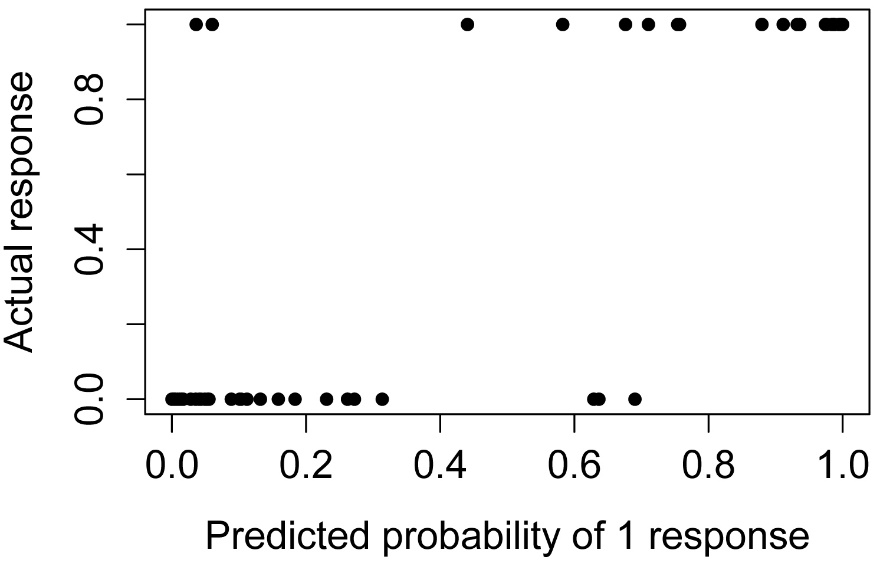
Simple plot of predicted values
### Create data frame with variables in
final model and NA’s omitted
library(dplyr)
Data.final =
select(Data,
Status,
Upland,
Migr,
Mass,
Indiv,
Insect,
Wood)
Data.final = na.omit(Data.final)
Data.final$predy = predict(model.final,
type="response")
plot(Status ~ predy,
data = Data.final,
pch = 16,
xlab="Predicted probability of 1 response",
ylab="Actual response")
Check for overdispersion
Overdispersion is a situation where the residual deviance of the glm is large relative to the residual degrees of freedom. These values are shown in the summary of the model. One guideline is that if the ratio of the residual deviance to the residual degrees of freedom exceeds 1.5, then the model is overdispersed. Overdispersion indicates that the model doesn’t fit the data well: the explanatory variables may not well describe the dependent variable or the model may not be specified correctly for these data. If there is overdispersion, one potential solution is to use the quasibinomial family option in glm.
summary(model.final)
Null deviance: 93.351 on 69 degrees of freedom
Residual deviance: 30.392 on 63 degrees of freedom
summary(model.final)$deviance / summary(model.final)$df.residual
[1] 0.482417
Alternative to assess models: using compare.glm
An alternative to, or a supplement to, using a stepwise procedure is comparing competing models with fit statistics. My compare.glm function will display AIC, AICc, BIC, and pseudo R-squared for glm models. The models used should all be fit to the same data. That is, caution should be used if different variables in the data set contain missing values. If you don’t have any preference on which fit statistic to use, I might recommend AICc, or BIC if you’d rather aim for having fewer terms in the final model.
A series of models can be compared with the standard anova function. Models should be nested within the previous model or the next model in the list in the anova function; and models should be fit to the same data. When comparing multiple regression models, a p-value to include a new term is often relaxed is 0.10 or 0.15.
In the following example, the models chosen with the stepwise procedure are used. Note that while model 9 minimizes AIC and AICc, model 8 minimizes BIC. The anova results suggest that model 8 is not a significant improvement to model 7. These results give support for selecting any of model 7, 8, or 9. Note that the SAS example in the Handbook selected model 4.
### Create data frame with just final
terms and no NA’s
library(dplyr)
Data.final =
select(Data,
Status,
Upland,
Migr,
Mass,
Indiv,
Insect,
Wood)
Data.final = na.omit(Data.final)
### Define models to compare.
model.1=glm(Status ~ 1,
data=Data.omit, family=binomial())
model.2=glm(Status ~ Release,
data=Data.omit, family=binomial())
model.3=glm(Status ~ Release + Upland,
data=Data.omit, family=binomial())
model.4=glm(Status ~ Release + Upland + Migr,
data=Data.omit, family=binomial())
model.5=glm(Status ~ Release + Upland + Migr + Mass,
data=Data.omit, family=binomial())
model.6=glm(Status ~ Release + Upland + Migr + Mass + Indiv,
data=Data.omit, family=binomial())
model.7=glm(Status ~ Release + Upland + Migr + Mass + Indiv + Insect,
data=Data.omit, family=binomial())
model.8=glm(Status ~ Upland + Migr + Mass + Indiv + Insect,
data=Data.omit, family=binomial())
model.9=glm(Status ~ Upland + Migr + Mass + Indiv + Insect + Wood,
data=Data.omit, family=binomial())
### Use compare.glm to assess fit statistics.
library(rcompanion)
compareGLM(model.1, model.2, model.3, model.4, model.5, model.6,
model.7, model.8, model.9)
$Models
Formula
1 "Status ~ 1"
2 "Status ~ Release"
3 "Status ~ Release + Upland"
4 "Status ~ Release + Upland + Migr"
5 "Status ~ Release + Upland + Migr + Mass"
6 "Status ~ Release + Upland + Migr + Mass + Indiv"
7 "Status ~ Release + Upland + Migr + Mass + Indiv + Insect"
8 "Status ~ Upland + Migr + Mass + Indiv + Insect"
9 "Status ~ Upland + Migr + Mass + Indiv + Insect + Wood"
$Fit.criteria
Rank Df.res AIC AICc BIC McFadden Cox.and.Snell Nagelkerke p.value
1 1 66 94.34 94.53 98.75 0.0000 0.0000 0.0000 Inf
2 2 65 62.13 62.51 68.74 0.3787 0.3999 0.5401 2.538e-09
3 3 64 56.02 56.67 64.84 0.4684 0.4683 0.6325 3.232e-10
4 4 63 51.63 52.61 62.65 0.5392 0.5167 0.6979 7.363e-11
5 5 62 50.64 52.04 63.87 0.5723 0.5377 0.7263 7.672e-11
6 6 61 49.07 50.97 64.50 0.6118 0.5618 0.7588 5.434e-11
7 7 60 46.42 48.90 64.05 0.6633 0.5912 0.7985 2.177e-11
8 6 61 44.71 46.61 60.14 0.6601 0.5894 0.7961 6.885e-12
9 7 60 44.03 46.51 61.67 0.6897 0.6055 0.8178 7.148e-12
### Use anova to compare each model to
the previous one.
anova(model.1, model.2, model.3,model.4, model.5, model.6,
model.7, model.8, model.9,
test="Chisq")
Analysis of Deviance Table
Model 1: Status ~ 1
Model 2: Status ~ Release
Model 3: Status ~ Release + Upland
Model 4: Status ~ Release + Upland + Migr
Model 5: Status ~ Release + Upland + Migr + Mass
Model 6: Status ~ Release + Upland + Migr + Mass + Indiv
Model 7: Status ~ Release + Upland + Migr + Mass + Indiv + Insect
Model 8: Status ~ Upland + Migr + Mass + Indiv + Insect
Model 9: Status ~ Upland + Migr + Mass + Indiv + Insect + Wood
Resid. Df Resid. Dev Df Deviance Pr(>Chi)
1 66 90.343
2 65 56.130 1 34.213 4.94e-09 ***
3 64 48.024 1 8.106 0.004412 **
4 63 41.631 1 6.393 0.011458 *
5 62 38.643 1 2.988 0.083872 .
6 61 35.070 1 3.573 0.058721 .
7 60 30.415 1 4.655 0.030970 *
8 61 30.710 -1 -0.295 0.587066
9 60 28.031 1 2.679 0.101686
Power analysis
See the Handbook for information on this topic.