An R Companion for the Handbook of Biological Statistics

Salvatore S. Mangiafico

One-way Anova

Examples in Summary and Analysis of Extension Program Evaluation

 

SAEPER: Introduction to Parametric Tests

SAEPER: One-way ANOVA
SAEPER: What are Least Square Means?

 

Packages used in this chapter

The following commands will install these packages if they are not already installed:

if(!require(dplyr)){install.packages("dplyr")}
if(!require(FSA)){install.packages("FSA")}
if(!require(car)){install.packages("car")}
if(!require(agricolae)){install.packages("agricolae")}
if(!require(multcomp)){install.packages("multcomp")}
if(!require(DescTools)){install.packages("DescTools")}
if(!require(lsmeans)){install.packages("lsmeans")}
if(!require(multcompView)){install.packages("multcompView")}
if(!require(Rmisc)){install.packages("Rmisc")}
if(!require(ggplot2)){install.packages("ggplot2")}
if(!require(pwr)){install.packages("pwr")}

 

When to use it

Analysis for this example is described below in the “How to do the test” section below.  

   

Null hypothesis

How the test works

Assumptions 

Additional analyses

See the Handbook for information on these topics.

 

Tukey-Kramer test

The Tukey mean separation tests and others are shown below in the “How to do the test” section.

 

Partitioning variance

This topic is not covered here.

 

Example

Code for this example is not included here.  An example is covered below in the “How to do the test” section.

 

Graphing the results

Graphing of the results is shown below in the “How to do the test” section.

 

Similar tests

Two-sample t–test, Two-way anova, Nested anova, Welch’s anova, and Kruskal–Wallis are presented elsewhere in this book. 

 

A permutation test, presented in the One-way Analysis with Permutation Test chapter, can also be employed as a nonparametric alternative.

 

How to do the test

The lm function in the native stats package fits a linear model by least squares, and can be used for a variety of analyses such as regression, analysis of variance, and analysis of covariance.  The analysis of variance is then conducted either with the Anova function in the car package for Type II or Type III sum of squares, or with the anova function in the native stats package for Type I sum of squares. 

 

If the analysis of variance indicates a significant effect of the independent variable, multiple comparisons among the levels of this factor can be conducted using Tukey or Least Significant Difference (LSD) procedures.  The problem of inflating the Type I Error Rate when making multiple comparisons is discussed in the Multiple Comparisons chapter in the Handbook.  R functions which make multiple comparisons usually allow for adjusting p-values.  In R, the “BH”, or “fdr”, procedure is the Benjamini–Hochberg procedure discussed in the Handbook.  See ?p.adjust for more information.

 

One-way anova example

 

### --------------------------------------------------------------
### One-way anova, SAS example, pp. 155-156
### --------------------------------------------------------------

Input =("
Location   Aam
Tillamook  0.0571
Tillamook  0.0813
Tillamook  0.0831
Tillamook  0.0976
Tillamook  0.0817
Tillamook  0.0859
Tillamook  0.0735
Tillamook  0.0659
Tillamook  0.0923
Tillamook  0.0836
Newport    0.0873
Newport    0.0662
Newport    0.0672
Newport    0.0819
Newport    0.0749
Newport    0.0649
Newport    0.0835
Newport    0.0725
Petersburg 0.0974
Petersburg 0.1352
Petersburg 0.0817
Petersburg 0.1016
Petersburg 0.0968
Petersburg 0.1064
Petersburg 0.1050
Magadan    0.1033
Magadan    0.0915
Magadan    0.0781
Magadan    0.0685
Magadan    0.0677
Magadan    0.0697
Magadan    0.0764
Magadan    0.0689
Tvarminne  0.0703
Tvarminne  0.1026 
Tvarminne  0.0956
Tvarminne  0.0973
Tvarminne  0.1039
Tvarminne  0.1045
")

Data = read.table(textConnection(Input),header=TRUE)

 

Specify the order of factor levels for plots and Dunnett comparison

 

library(dplyr)

Data =
mutate(Data,
       Location = factor(Location, levels=unique(Location)))

 

Produce summary statistics

library(FSA)  

Summarize(Aam ~ Location,
           data=Data,
           digits=3)

    Location  n  mean    sd   min    Q1 median    Q3   max
1  Tillamook 10 0.080 0.012 0.057 0.075  0.082 0.085 0.098
2    Newport  8 0.075 0.009 0.065 0.067  0.074 0.082 0.087
3 Petersburg  7 0.103 0.016 0.082 0.097  0.102 0.106 0.135
4    Magadan  8 0.078 0.013 0.068 0.069  0.073 0.081 0.103
5  Tvarminne  6 0.096 0.013 0.070 0.096  0.100 0.104 0.104

Fit the linear model and conduct ANOVA

 

model = lm(Aam ~ Location,
           data=Data)

library(car)

Anova(model, type="II")                    # Can use type="III"

   ### If you use type="III", you need the following line before the analysi
   ### options(contrasts = c("contr.sum", "contr.poly"))

 

             Sum Sq Df F value    Pr(>F)   

Location  0.0045197  4   7.121 0.0002812 ***

Residuals 0.0053949 34                     

 

 

anova(model)                               # Produces type I sum of squares

 

          Df    Sum Sq    Mean Sq F value    Pr(>F)   

Location   4 0.0045197 0.00112992   7.121 0.0002812 ***

Residuals 34 0.0053949 0.00015867  

 

 

summary(model)     # Produces r-square, overall p-value, parameter estimates

 

Multiple R-squared:  0.4559,  Adjusted R-squared:  0.3918

F-statistic: 7.121 on 4 and 34 DF,  p-value: 0.0002812

 

 

Checking assumptions of the model

hist(residuals(model),
     col="darkgray")

A histogram of residuals from a linear model.  The distribution of these residuals should be approximately normal.

plot(fitted(model),
     residuals(model))

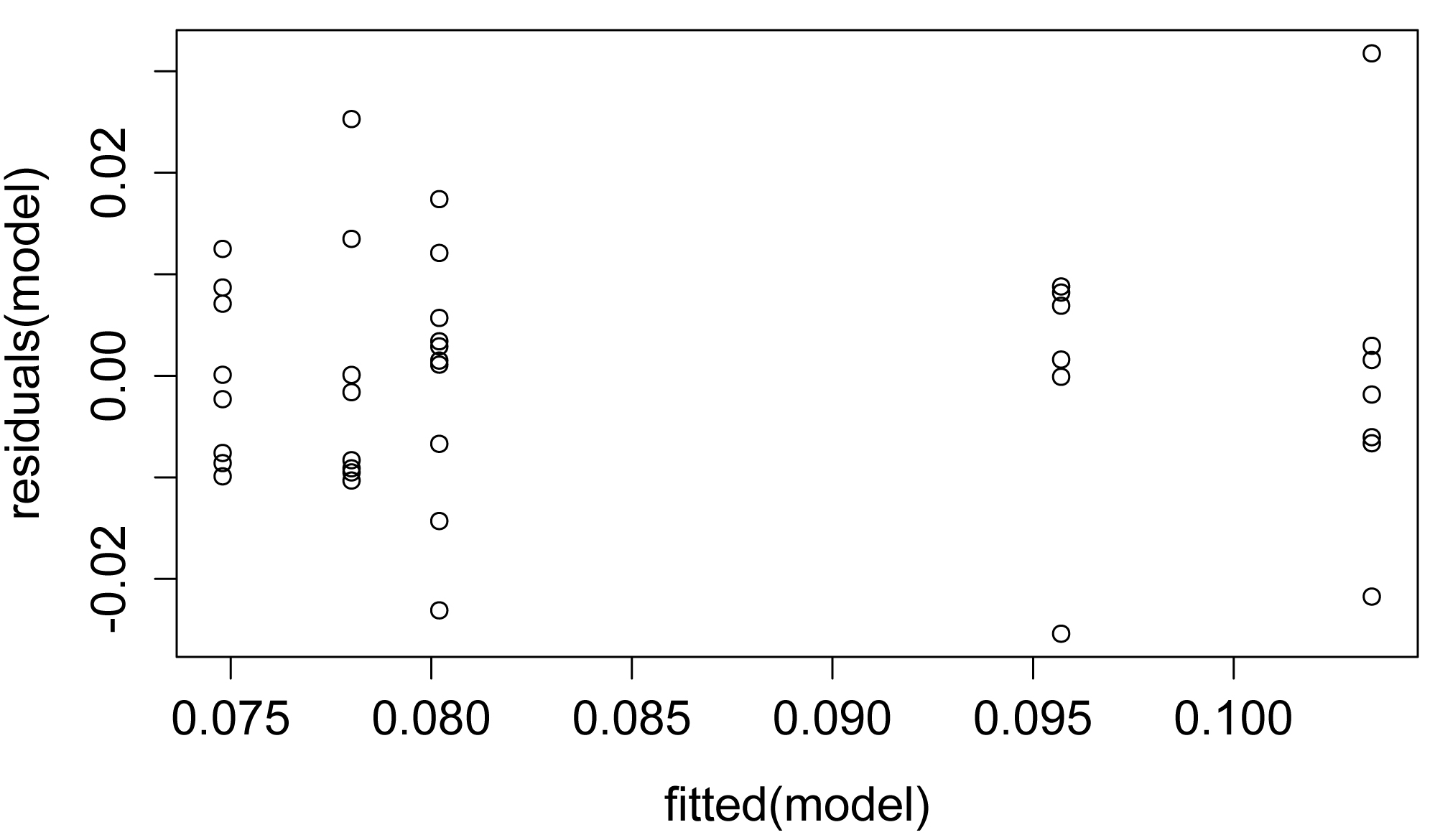
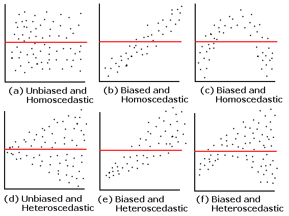
A plot of residuals vs. predicted values.  The residuals should be unbiased and homoscedastic.  For an illustration of these properties, see this diagram by Steve Jost at DePaul University: condor.depaul.edu/sjost/it223/documents/resid-plots.gif.

 

 

### additional model checking plots with: plot(model)
### alternative: library(FSA); residPlot(model) 

 

 

Tukey and Least Significant Difference mean separation tests (pairwise comparisons)

Tukey and other multiple comparison tests can be performed with a handful of functions.  The functions TukeyHSD, HSD.test, and LSD.test are probably not appropriate for cases where there are unbalanced data or unequal variances among levels of the factor, though TukeyHSD does make an adjustment for mildly unbalanced data.  It is my understanding that the multcomp and lsmeans packages are more appropriate for unbalanced data.  Another alternative is the DTK package that performs mean separation tests on data with unequal sample sizes and no assumption of equal variances.

 

Tukey comparisons in agricolae package

library(agricolae)

(HSD.test(model, "Location"))          # outer parentheses print result

         trt     means  M
1 Petersburg 0.1034429  a
2 Tvarminne  0.0957000 ab
3 Tillamook  0.0802000 bc
4 Magadan    0.0780125 bc
5 Newport    0.0748000  c

# Means sharing the same letter are not significantly different

LSD comparisons in agricolae package

library(agricolae)

(LSD.test(model, "Location",   # outer parentheses print result
           alpha = 0.05,      
           p.adj="none"))      # see ?p.adjust for options

         trt     means M
1 Petersburg 0.1034429 a
2 Tvarminne  0.0957000 a
3 Tillamook  0.0802000 b
4 Magadan    0.0780125 b
5 Newport    0.0748000 b

# Means sharing the same letter are not significantly different

Multiple comparisons in multcomp package

Note that “Tukey” here does not mean Tukey-adjusted comparisons.  It just sets up a matrix to compare each mean to each other mean.

library(multcomp)

mc = glht(model,
          mcp(Location = "Tukey"))

mcs = summary(mc, test=adjusted("single-step"))

mcs

   ### Adjustment options: "none", "single-step", "Shaffer",
   ###                     "Westfall", "free", "holm", "hochberg",
   ###                     "hommel", "bonferroni", "BH", "BY", "fdr"

Linear Hypotheses:

                             Estimate Std. Error t value Pr(>|t|)   

Newport - Tillamook == 0    -0.005400   0.005975  -0.904  0.89303   

Petersburg - Tillamook == 0  0.023243   0.006208   3.744  0.00555 **

Magadan - Tillamook == 0    -0.002188   0.005975  -0.366  0.99596   

Tvarminne - Tillamook == 0   0.015500   0.006505   2.383  0.14413   

Petersburg - Newport == 0    0.028643   0.006519   4.394  < 0.001 ***

Magadan - Newport == 0       0.003213   0.006298   0.510  0.98573   

Tvarminne - Newport == 0     0.020900   0.006803   3.072  0.03153 * 

Magadan - Petersburg == 0   -0.025430   0.006519  -3.901  0.00376 **

Tvarminne - Petersburg == 0 -0.007743   0.007008  -1.105  0.80211   

Tvarminne - Magadan == 0     0.017688   0.006803   2.600  0.09254 . 

 

 

cld(mcs,
    level=0.05,
    decreasing=TRUE)

 

Tillamook    Newport Petersburg    Magadan  Tvarminne

      "bc"        "c"        "a"       "bc"       "ab"

 

    ### Means sharing a letter are not significantly different

 

Multiple comparisons to a control in multcomp package

 

### Control is the first level of the factor

library(multcomp)

mc = glht(model,
          mcp(Location = "Dunnett"))

summary(mc, test=adjusted("single-step"))

   ### Adjustment options: "none", "single-step", "Shaffer",
   ###                     "Westfall", "free", "holm", "hochberg",
   ###                     "hommel", "bonferroni", "BH", "BY", "fdr"

Linear Hypotheses:

                             Estimate Std. Error t value Pr(>|t|)  

Newport - Tillamook == 0    -0.005400   0.005975  -0.904  0.79587  

Petersburg - Tillamook == 0  0.023243   0.006208   3.744  0.00252 **

Magadan - Tillamook == 0    -0.002188   0.005975  -0.366  0.98989  

Tvarminne - Tillamook == 0   0.015500   0.006505   2.383  0.07794 .

 

 

Multiple comparisons to a control with Dunnett Test

 

### The control group can be specified with the control option,
###   or will be the first level of the factor

library(DescTools)

DunnettTest(Aam ~ Location,
            data = Data)

 

  Dunnett's test for comparing several treatments with a control : 

    95% family-wise confidence level

 

                            diff       lwr.ci     upr.ci   pval   

Newport-Tillamook    -0.00540000 -0.020830113 0.01003011 0.7958   

Petersburg-Tillamook  0.02324286  0.007212127 0.03927359 0.0026 **

Magadan-Tillamook    -0.00218750 -0.017617613 0.01324261 0.9899   

Tvarminne-Tillamook   0.01550000 -0.001298180 0.03229818 0.0778 .

 

 

Multiple comparisons with least square means

Least square means can be calculated for each group.  Here a Tukey adjustment is applied for multiple comparisons among group least square means.  The multiple comparisons can be displayed as a compact letter display.

library(lsmeans)
library(multcompView)

leastsquare = lsmeans(model,
                      pairwise ~ Location,
                      adjust = "tukey")

 

$contrasts

 contrast                   estimate          SE df t.ratio p.value

 Tillamook - Newport     0.005400000 0.005975080 34   0.904  0.8935

 Tillamook - Petersburg -0.023242857 0.006207660 34  -3.744  0.0057

 Tillamook - Magadan     0.002187500 0.005975080 34   0.366  0.9960

 Tillamook - Tvarminne  -0.015500000 0.006504843 34  -2.383  0.1447

 Newport - Petersburg   -0.028642857 0.006519347 34  -4.394  0.0009

 Newport - Magadan      -0.003212500 0.006298288 34  -0.510  0.9858

 Newport - Tvarminne    -0.020900000 0.006802928 34  -3.072  0.0317

 Petersburg - Magadan    0.025430357 0.006519347 34   3.901  0.0037

 Petersburg - Tvarminne  0.007742857 0.007008087 34   1.105  0.8028

 Magadan - Tvarminne    -0.017687500 0.006802928 34  -2.600  0.0929

 

P value adjustment: tukey method for comparing a family of 5 estimates

 

 

cld(leastsquare,
    alpha   = 0.05,
    Letters = letters,
    adjust="tukey")
   

 

Location      lsmean          SE df   lower.CL   upper.CL .group

 Newport    0.0748000 0.004453562 34 0.06268565 0.08691435  a   

 Magadan    0.0780125 0.004453562 34 0.06589815 0.09012685  ab  

 Tillamook  0.0802000 0.003983387 34 0.06936459 0.09103541  ab  

 Tvarminne  0.0957000 0.005142530 34 0.08171155 0.10968845   bc 

 Petersburg 0.1034429 0.004761058 34 0.09049207 0.11639365    c 

 

Confidence level used: 0.95

Conf-level adjustment: sidak method for 5 estimates

P value adjustment: tukey method for comparing a family of 5 estimates

significance level used: alpha = 0.05

 

 

Graphing the results

 

Simple box plots of values across groups

 

boxplot(Aam ~ Location,
        data = Data,
        ylab="aam / height",
        xlab="Location")

 

 

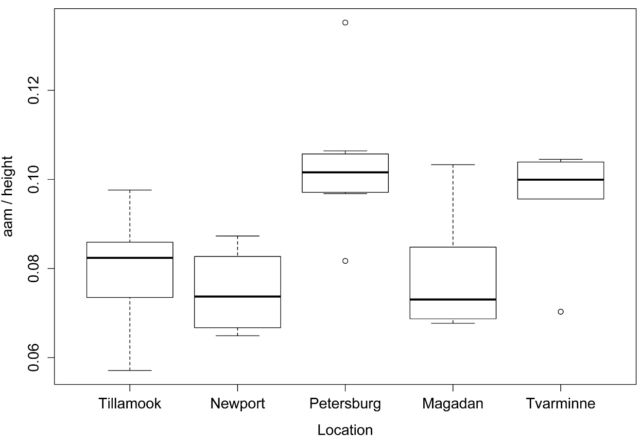
Box plots of values for each level of the independent variable for a one-way analysis of variance (ANOVA).

 

 

Simple bar plot of means across groups

 

### Summarize the data frame (Data) into a table

library(Rmisc)  

Data2 = summarySE(data=Data,
          "Aam",
          groupvars="Location",
          conf.interval = 0.95)

Tabla = as.table(Data2$Aam)         
rownames(Tabla) = Data2$Location

Tabla

 

Tillamook    Newport Petersburg    Magadan  Tvarminne

 0.0802000  0.0748000  0.1034429  0.0780125  0.0957000

 

 

barplot(Tabla,
        ylab="aam / height",
        xlab="Location")

 

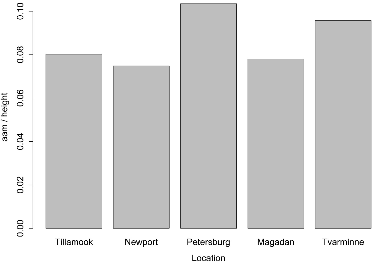
Bar plot of means for each level of the independent variable for a one-way analysis of variance (ANOVA).

 

 

Bar plot of means with error bars across groups

 

library(ggplot2)

offset.v = -3     # offsets for mean letters
offset.h = 0.5

ggplot(Data2,
       aes(x = Location, y = Aam,
           ymax=0.12, ymin=0.0))  +
       geom_bar(stat="identity", fill="gray50",
           colour = "black", width = 0.7)  +
       geom_errorbar(aes(ymax=Aam+se, ymin=Aam-se),
                     width=0.0, size=0.5, color="black")  +
       geom_text(aes(label=c("bc","c","a","bc","ab"),
                 hjust=offset.h, vjust=offset.v)) +             
       labs(x = "Sample location",
            y = "aam / height")  +
       ## ggtitle("Main title") +
       theme_bw()  +
       theme(panel.grid.major.x = element_blank(),
             panel.grid.major.y = element_line(colour = "grey80"),
             plot.title = element_text(size = rel(1.5),
             face = "bold", vjust = 1.5),
             axis.title = element_text(face = "bold"),
             axis.title.y = element_text(vjust= 1.8),
             axis.title.x = element_text(vjust= -0.5),
             panel.border = element_rect(colour="black")
             )

 

 

Bar plot of means for each level of the independent variable of a one-way analysis of variance (ANOVA).  Error indicates standard error of the mean.  Bars sharing the same letter are not significantly different according to Tukey’s HSD test.

 

 

Welch’s anova

Bartlett’s test and Levene’s test can be used to check the homoscedasticity of groups from a one-way anova.  A significant result for these tests (p < 0.05) suggests that groups are heteroscedastic.  One approach with heteroscedastic data in a one way anova is to use the Welch correction with the oneway.test function in the native stats package.  A more versatile approach is to use the white.adjust=TRUE option in the Anova function from the car package.

### Bartlett test for homogeneity of variance

bartlett.test(Aam ~ Location,
       data = Data) 

 

Bartlett test of homogeneity of variances

 

Bartlett's K-squared = 2.4341, df = 4, p-value = 0.6565

 

 

### Levene test for homogeneity of variance

library(car)

leveneTest(Aam ~ Location,
           data = Data) 

 

Levene's Test for Homogeneity of Variance (center = median)

 

      Df F value Pr(>F)

group  4    0.12 0.9744

      34 

 

 

### Welch’s anova for unequal variances

oneway.test(Aam ~ Location,
            data=Data,
            var.equal=FALSE)

 

One-way analysis of means (not assuming equal variances)

 

F = 5.6645, num df = 4.000, denom df = 15.695, p-value = 0.00508

 

 

### White-adjusted anova for heteroscedasticity

model = lm(Aam ~ Location,
           data=Data)

library(car)

Anova(model, Type="II",
      white.adjust=TRUE)

 

          Df      F   Pr(>F)  

Location   4 5.4617 0.001659 **

Residuals 34                  

 

#     #     #

 

 

Power analysis

Power analysis for one-way anova

 

### --------------------------------------------------------------
### Power analysis for anova, pp. 157
### --------------------------------------------------------------

library(pwr)
 
groups = 5
means = c(10, 10, 15, 15, 15)
sd = 12

grand.mean  = mean(means)
Cohen.f = sqrt( sum( (1/groups) * (means-grand.mean)^2) ) /sd

pwr.anova.test(k = groups,
               n = NULL,
               f = Cohen.f,
               sig.level = 0.05,
               power = 0.80)

 

Balanced one-way analysis of variance power calculation

 

        n = 58.24599

 

NOTE: n is number in each group

 

 

#     #     #

 

©2015 by Salvatore S. Mangiafico.
Rutgers Cooperative Extension, New Brunswick, NJ.

Organization of statistical tests and selection of examples for these tests ©2014 by John H. McDonald.  Used with permission.

Non-commercial reproduction of this content, with attribution, is permitted.  For-profit reproduction without permission is prohibited.

If you use the code or information in this site in a published work, please cite it as a source.  Also, if you are an instructor and use this book in your course, please let me know.   My contact information is on the About the Author page.

Citation:

Mangiafico, S.S. 2015. An R Companion for the Handbook of Biological Statistics, version 1.3.9, revised 2023.
rcompanion.org/rcompanion/. (Pdf version: rcompanion.org/documents/RCompanionBioStatistics.pdf.)