Python Handbook: One-sample Wilcoxon Signed Rank Test

One-sample Wilcoxon signed rank test in SAEPER

For a discussion of this test, see the corresponding chapter in Summary and Analysis of Extension Program Evaluation in R (rcompanion.org/handbook/F_02.html).

Importing packages in this chapter

The following commands will import required packages used in this chapter from libraries and assign them common aliases. You may need install these libraries first.

import io

import os

import scipy.stats as stats

import pandas as pd

import pingouin as pg

import matplotlib.pyplot as plt

import seaborn as sns

Setting your working directory

You may wish to set your working directory for exported plots.

os.chdir("C:/Users/Sal Mangiafico/Desktop")

print(os.getcwd())

Example of the one-sample Wilcoxon signed rank test

Data = pd.read_table(sep="\\s+", filepath_or_buffer=io.StringIO("""
Speaker          Rater Likert
"Maggie Simpson"   1         3
"Maggie Simpson"   2         4
"Maggie Simpson"   3         5
"Maggie Simpson"   4         4
"Maggie Simpson"   5         4
"Maggie Simpson"   6         4
"Maggie Simpson"   7         4
"Maggie Simpson"   8         3
"Maggie Simpson"   9         2
"Maggie Simpson" 10         5
"""))

### Convert Instructor and Location to category type

Data['Speaker'] = Data['Speaker'].astype('category')

### Create new variable, Likert as a category variable, and add '1' level

Data['Likert.f'] = Data['Likert'].astype('category')

Data['Likert.f'] = Data ['Likert.f'].cat.add_categories(1)

LikertLevels =[1, 2, 3, 4, 5]

Data['Likert.f'] = Data['Likert.f'].cat.reorder_categories(LikertLevels)

### Display some summary statistics for the data frame

print(Data.info())

# Column Non-Null Count Dtype

--- ------ -------------- -----

0 Speaker 10 non-null category

1 Rater 10 non-null int64

2 Likert 10 non-null int64

3 Likert.f 10 non-null category

print(Data['Speaker'].cat.categories)

Index(['Maggie Simpson''], dtype='object')

print(Data['Likert.f'].cat.categories)

Index([1, 2, 3, 4, 5], dtype='int64')

Summarize data treating Likert scores as factors

Note that the variable we want to count is Likert.f, which is a category variable. Counts for Likert.f are tabulated over values of Speaker. The normalize=True option reports proportions. If sort=True, the results will be ordered by which categories have the most observations.

Data['Likert.f'].value_counts(sort=False)

Likert.f

1 0

2 1

3 2

4 5

5 2

Data['Likert.f'].value_counts(sort=False, normalize=True)

Likert.f

1 0.0

2 0.1

3 0.2

4 0.5

5 0.2

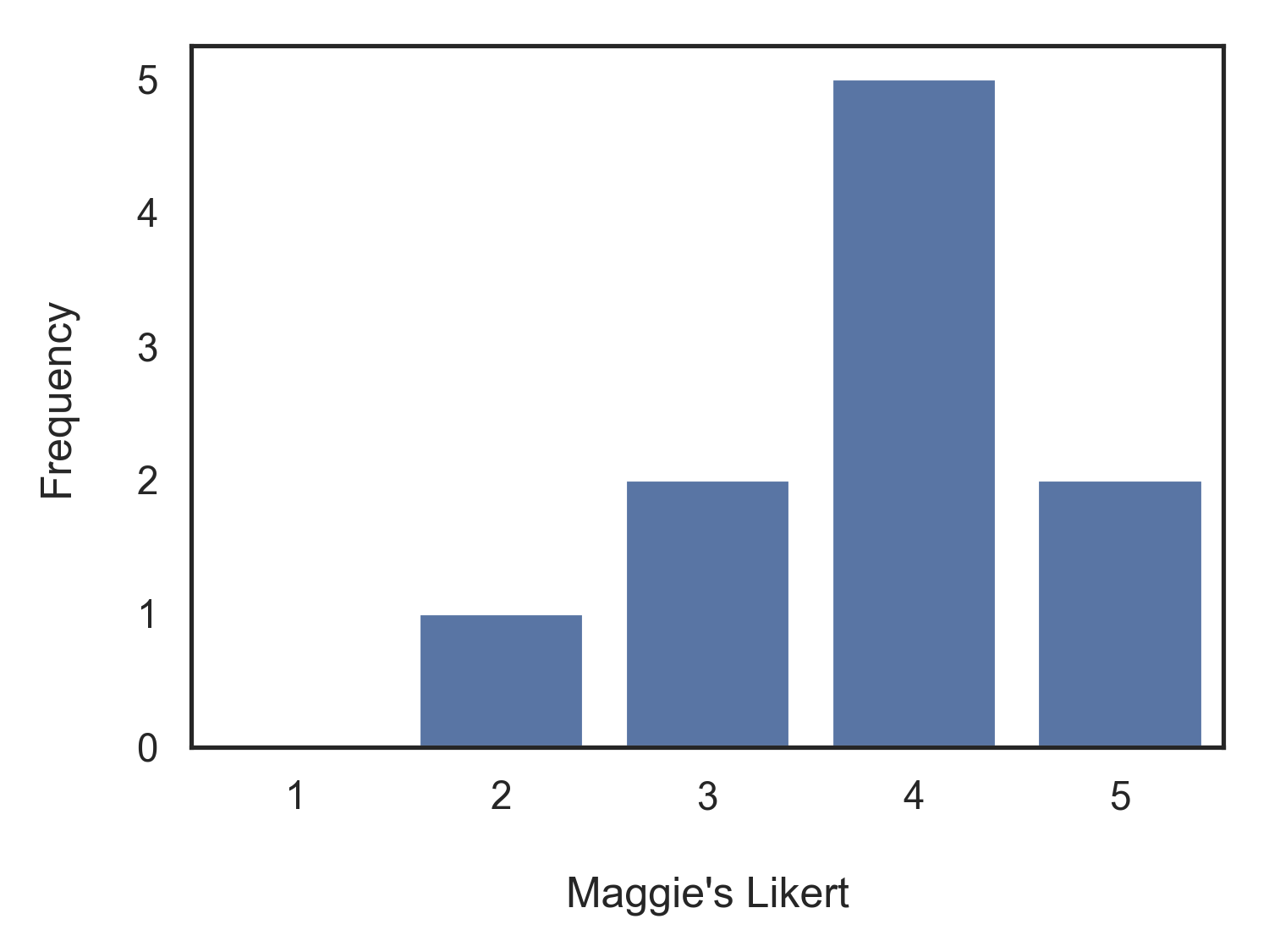
Bar plot

Simple seaborn call

sns.countplot(data=Data, x="Likert.f")

Formatting and export as file

sns.set_theme(style='white')

plt.figure(figsize=(5, 3.75))

sns.countplot(data=Data, x="Likert.f")

plt.title('')

plt.xlabel("\nMaggie's Likert")

plt.ylabel('Frequency\n')

plt.tight_layout()

plt.savefig('MaggieLikert.png', format='png', dpi=300)

plt.show()

Histogram of bootstrapped means

Summarize data treating Likert scores as numeric

Summary = Data.groupby('Speaker')['Likert'].describe()

print(Summary)

count mean std min 25% 50% 75% max

Speaker

Maggie Simpson 10.0 3.8 0.918937 2.0 3.25 4.0 4.0 5.0

One-sample Wilcoxon signed-rank test

Using pingouin

As far as I can tell, you have to manually subtract mu, the point of central tendency under the null hypothesis, if it’s not 0.

mu = 3

pg.wilcoxon(Data['Likert'] - mu)

W-val alternative p-val RBC CLES

Wilcoxon 3.5 two-sided 0.040067 0.805556 NaN

Note that the effect size statistic, rank biserial correlation coefficient, RBC, is reported by default.

Using pysci.stats

Note, that the continuty correction is not used by default, whereas it is used by default in pingouin.