![[banner]](images/banner.jpg "Piney Point, Sunset Lake, Bridgeton, New Jersey")
Friedman test in SAEPER
For a discussion of this test, see the corresponding chapter in Summary and Analysis of Extension Program Evaluation in R (rcompanion.org/handbook/F_10.html).
Importing packages in this chapter
The following commands will import required packages used in this chapter from libraries and assign them common aliases. You may need install these libraries first.
import io
import os
import numpy as np
import scipy.stats as stats
import pandas as pd
import pingouin as pg
import scikit_posthocs as sp
import matplotlib.pyplot as plt
import seaborn as sns
Setting your working directory
You may wish to set your working directory for exported plots.
os.chdir("C:/Users/Sal Mangiafico/Desktop")
print(os.getcwd())
Example of Friedman test
Data = pd.read_table(sep="\\s+", filepath_or_buffer=io.StringIO("""
Instructor Rater Likert
"Bob Belcher" a 4
"Bob Belcher" b 5
"Bob Belcher" c 4
"Bob Belcher" d 6
"Bob Belcher" e 6
"Bob Belcher" f 6
"Bob Belcher" g 10
"Bob Belcher" h 6
"Linda Belcher" a 8
"Linda Belcher" b 6
"Linda Belcher" c 8
"Linda Belcher" d 8
"Linda Belcher" e 8
"Linda Belcher" f 7
"Linda Belcher" g 10
"Linda Belcher" h 9
"Tina Belcher" a 7
"Tina Belcher" b 5
"Tina Belcher" c 7
"Tina Belcher" d 8
"Tina Belcher" e 8
"Tina Belcher" f 9
"Tina Belcher" g 10
"Tina Belcher" h 9
"Gene Belcher" a 6
"Gene Belcher" b 4
"Gene Belcher" c 5
"Gene Belcher" d 5
"Gene Belcher" e 6
"Gene Belcher" f 6
"Gene Belcher" g 5
"Gene Belcher" h 5
"Louise Belcher" a 8
"Louise Belcher" b 7
"Louise Belcher" c 8
"Louise Belcher" d 8
"Louise Belcher" e 9
"Louise Belcher" f 9
"Louise Belcher" g 8
"Louise Belcher" h 10
"""))
### Convert Instructor and Rater to category type
Data['Instructor'] = Data['Instructor'].astype('category')
Data['Rater'] = Data['Rater'].astype('category')
### Create new variable, Likert as a category variable
Data['Likert.f'] = Data['Likert'].astype('category')
### Order Speaker by desired values
InstructorLevels = ['Bob Belcher', 'Linda Belcher', 'Tina Belcher',
'Gene Belcher', 'Louise Belcher']
Data['Instructor'] = Data['Instructor'].cat.reorder_categories(InstructorLevels)
print(Data['Instructor'].cat.categories)
Index(['Bob Belcher', 'Linda Belcher', 'Tina Belcher', 'Gene Belcher',
'Louise Belcher'],
dtype='object')
print(Data.info())
# Column Non-Null Count Dtype
--- ------ -------------- -----
0 Instructor 40 non-null category
1 Rater 40 non-null category
2 Likert 40 non-null int64
3 Likert.f 40 non-null category
Summarize data treating Likert scores as categories
pd.crosstab(Data['Instructor'], Data['Likert.f'])
Likert.f 4 5 6 7 8 9 10
Instructor
Bob Belcher 2 1 4 0 0 0 1
Linda Belcher 0 0 1 1 4 1 1
Tina Belcher 0 1 0 2 2 2 1
Gene Belcher 1 4 3 0 0 0 0
Louise Belcher 0 0 0 1 4 2 1
pd.crosstab(Data['Instructor'], Data['Likert.f'], normalize='index')
Likert.f 4 5 6 7 8 9 10
Instructor
Bob Belcher 0.250 0.125 0.500 0.000 0.00 0.000 0.125
Linda Belcher 0.000 0.000 0.125 0.125 0.50 0.125 0.125
Tina Belcher 0.000 0.125 0.000 0.250 0.25 0.250 0.125
Gene Belcher 0.125 0.500 0.375 0.000 0.00 0.000 0.000
Louise Belcher 0.000 0.000 0.000 0.125 0.50 0.250 0.125
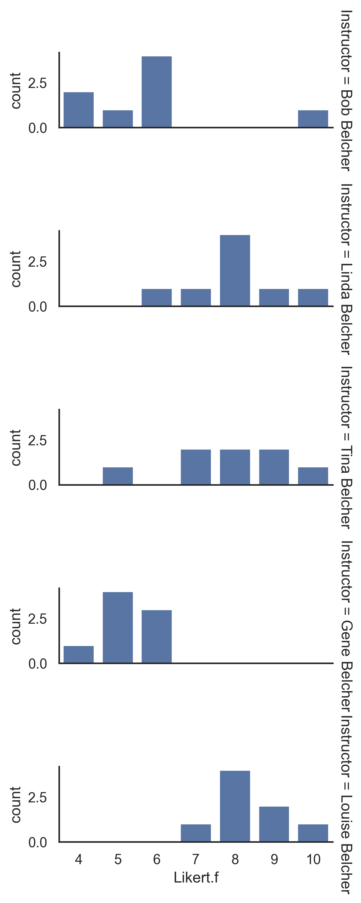
Bar plots of data by group
sns.set_theme(style='white')
Plot = sns.FacetGrid(data=Data, row='Instructor',
margin_titles=True, height=2, aspect= 2)
Plot.map(sns.countplot, 'Likert.f')
Plot.tight_layout()
Plot.savefig('LikertBarBelcher.png', format='png', dpi=300)
Summarize data treating Likert scores as numeric
Summary = Data.groupby('Instructor')['Likert'].describe()
print(Summary)
count mean std min 25% 50% 75% max
Instructor
Bob Belcher 8.0 5.875 1.885092 4.0 4.75 6.0 6.00 10.0
Linda Belcher 8.0 8.000 1.195229 6.0 7.75 8.0 8.25 10.0
Tina Belcher 8.0 7.875 1.552648 5.0 7.00 8.0 9.00 10.0
Gene Belcher 8.0 5.250 0.707107 4.0 5.00 5.0 6.00 6.0
Louise Belcher 8.0 8.375 0.916125 7.0 8.00 8.0 9.00 10.0
Friedman test example
Using pingouin
pg.friedman(data=Data, dv="Likert", within="Instructor", subject="Rater")
Source W ddof1 Q p-unc
Friedman Instructor 0.72309 4 23.138889 0.000119
### Note that the effective size statistic, Kendall’s W, is included in the output.
Using pysci.stats
Bob = np.array(Data['Likert'][Data['Instructor']== 'Bob Belcher'])
Linda = np.array(Data['Likert'][Data['Instructor']== 'Linda Belcher'])
Tina = np.array(Data['Likert'][Data['Instructor']== 'Tina Belcher'])
Gene = np.array(Data['Likert'][Data['Instructor']== 'Gene Belcher'])
Louise = np.array(Data['Likert'][Data['Instructor']== 'Louise Belcher'])
stats.friedmanchisquare(Bob, Linda, Tina, Gene, Louise)
FriedmanchisquareResult(statistic=23.138888888888907, pvalue=0.00011878735218879764)
Stat, Pvalue = stats.friedmanchisquare(Bob, Linda, Tina, Gene, Louise)
round(Stat, 3)
23.139
round(Pvalue, 6)
0.000119
Post-hoc tests for multiple comparisons of groups
Some results below differ from those reported by R. This may have to do with differences p-value adjustment methods. For similar tests, with the p_adjust=None option, the results will be the same as the test in R using the p.adjust.method="none" option.
The following call will prevent pandas from truncating the output.
pd.set_option('display.max_columns', 500)
The following will order the Instructor categories by their median responses. It appears, though, that this ordering isn’t used in the following post-hoc functions.
InstructorLevels = ['Linda Belcher', 'Louise Belcher','Tina Belcher',
'Bob Belcher','Gene Belcher']
Data['Instructor'] = Data['Instructor'].cat.reorder_categories(InstructorLevels)
print(Data['Instructor'].cat.categories)
Index(['Linda Belcher', 'Louise Belcher', 'Tina Belcher', 'Bob Belcher',
'Gene Belcher'],
dtype='object')
Conover test
Several different p-value adjustment methods are available. See the function documentation for the options.
sp.posthoc_conover_friedman(Data, melted=True,
y_col='Likert', group_col='Instructor',
block_col='Rater', block_id_col='Rater',
p_adjust=None)
Bob Belcher Linda Belcher Tina Belcher Gene Belcher Louise Belcher
Bob Belcher 1.000000 0.000085 0.000925 1.932115e-01 4.987865e-06
Linda Belcher 0.000085 1.000000 0.381682 2.237578e-06 3.086386e-01
Tina Belcher 0.000925 0.381682 1.000000 2.509627e-05 6.434725e-02
Gene Belcher 0.193212 0.000002 0.000025 1.000000e+00 1.433972e-07
Louise Belcher 0.000005 0.308639 0.064347 1.433972e-07 1.000000e+00
Nemenyi test
sp.posthoc_nemenyi_friedman(Data, melted=True,
y_col='Likert', group_col='Instructor',
block_col='Rater', block_id_col='Rater')
Bob Belcher Linda Belcher Tina Belcher Gene Belcher Louise Belcher
Bob Belcher 1.000000 0.102135 0.277518 0.953951 0.022372
Linda Belcher 0.102135 1.000000 0.989665 0.013570 0.981551
Tina Belcher 0.277518 0.989665 1.000000 0.055728 0.842625
Gene Belcher 0.953951 0.013570 0.055728 1.000000 0.001894
Louise Belcher 0.022372 0.981551 0.842625 0.001894 1.000000
Siegel test
Several different p-value adjustment methods are available. See the function documentation for the options.
sp.posthoc_siegel_friedman(Data, melted=True,
y_col='Likert', group_col='Instructor',
block_col='Rater', block_id_col='Rater',
p_adjust=None)
Bob Belcher Linda Belcher Tina Belcher Gene Belcher Louise Belcher
Bob Belcher 1.000000 0.014255 0.048107 0.476767 0.002663
Linda Belcher 0.014255 1.000000 0.635256 0.001565 0.579991
Tina Belcher 0.048107 0.635256 1.000000 0.007190 0.304072
Gene Belcher 0.476767 0.001565 0.007190 1.000000 0.000203
Louise Belcher 0.002663 0.579991 0.304072 0.000203 1.000000
Miller test
sp.posthoc_miller_friedman(Data, melted=True,
y_col='Likert', group_col='Instructor',
block_col='Rater', block_id_col='Rater')
Bob Belcher Linda Belcher Tina Belcher Gene Belcher Louise Belcher
Bob Belcher 1.000000 0.198682 0.418842 0.972890 0.060478
Linda Belcher 0.198682 1.000000 0.994127 0.040428 0.989407
Tina Belcher 0.418842 0.994127 1.000000 0.124465 0.901150
Gene Belcher 0.972890 0.040428 0.124465 1.000000 0.007940
Louise Belcher 0.060478 0.989407 0.901150 0.007940 1.000000
Example from Conover
This example is taken from the Friedman test section of Conover (1999). Note, here, that the data aren’t in long format, but in wide format. For data in this format, the easiest thing to subset the data into a data frame called Conover1, with just the columns of observations.
Conover = pd.read_table(sep="\\s+", filepath_or_buffer=io.StringIO("""
Homeowner Grass1 Grass2 Grass3 Grass4
1 4 3 2 1
2 4 2 3 1
3 3 1.5 1.5 4
4 3 1 2 4
5 4 2 1 3
6 2 2 2 4
7 1 3 2 4
8 2 4 1 3
9 3.5 1 2 3.5
10 4 1 3 2
11 4 2 3 1
12 3.5 1 2 3.5
"""))
Columns = ['Grass1', 'Grass2', 'Grass3', 'Grass4']
Conover1 = Conover[Columns]
Conover1
Grass1 Grass2 Grass3 Grass4
0 4.0 3.0 2.0 1.0
1 4.0 2.0 3.0 1.0
2 3.0 1.5 1.5 4.0
3 3.0 1.0 2.0 4.0
4 4.0 2.0 1.0 3.0
5 2.0 2.0 2.0 4.0
6 1.0 3.0 2.0 4.0
7 2.0 4.0 1.0 3.0
8 3.5 1.0 2.0 3.5
9 4.0 1.0 3.0 2.0
10 4.0 2.0 3.0 1.0
11 3.5 1.0 2.0 3.5
pg.friedman(Conover1)
Source W ddof1 Q p-unc
Friedman Within 0.224926 3 8.097345 0.044042
sp.posthoc_conover_friedman(Conover1)
Grass1 Grass2 Grass3 Grass4
Grass1 1.000000 0.014895 0.022603 0.483434
Grass2 0.014895 1.000000 0.860437 0.071737
Grass3 0.022603 0.860437 1.000000 0.101742
References
Conover, W.J. 1999. Practical Nonparametric Statistics, 3rd. John Wiley & Sons.