![[banner]](images/banner.jpg "Piney Point, Sunset Lake, Bridgeton, New Jersey")
Confidence intervals in SAEPER
For a discussion of the following topics, see the corresponding chapter in Summary and Analysis of Extension Program Evaluation in R (rcompanion.org/handbook/C_03.html).
• Understanding confidence intervals
Importing packages in this chapter
The following commands will import required packages used in this chapter from libraries and assign them common aliases. You may need install these libraries first.
import io
import os
import numpy as np
import scipy.stats as stats
import pandas as pd
import statsmodels.stats.api as sms
import researchpy as rp
import seaborn as sns
import matplotlib.pyplot as plt
Setting your working directory
You may wish to set your working directory for exported plots.
os.chdir("C:/Users/Sal Mangiafico/Desktop")
print(os.getcwd())
Example for confidence intervals
For this example, extension educators had students wear pedometers to count their number of steps over the course of a day. The following data are the result. Rating is the rating each student gave about the usefulness of the program, on a 1-to-10 scale.
Data = pd.read_table(sep="\\s+", filepath_or_buffer=io.StringIO("""
Student Gender Teacher Steps Rating
a female Catbus 8000 7
b female Catbus 9000 10
c female Catbus 10000 9
d female Catbus 7000 5
e female Catbus 6000 4
f female Catbus 8000 8
g male Catbus 7000 6
h male Catbus 5000 5
i male Catbus 9000 10
j male Catbus 7000 8
k female Satsuki 8000 7
l female Satsuki 9000 8
m female Satsuki 9000 8
n female Satsuki 8000 9
o male Satsuki 6000 5
p male Satsuki 8000 9
q male Satsuki 7000 6
r female Totoro 10000 10
s female Totoro 9000 10
t female Totoro 8000 8
u female Totoro 8000 7
v female Totoro 6000 7
w male Totoro 6000 8
x male Totoro 8000 10
y male Totoro 7000 7
z male Totoro 7000 7
"""))
print(Data.info())
# Column Non-Null Count Dtype
--- ------ -------------- -----
0 Student 26 non-null object
1 Gender 26 non-null object
2 Teacher 26 non-null object
3 Steps 26 non-null int64
4 Rating 26 non-null int64
dtypes: int64(2), object(3)
print(Data.describe())
Steps Rating
count 26.000000 26.000000
mean 7692.307692 7.615385
std 1289.006773 1.745323
min 5000.000000 4.000000
25% 7000.000000 7.000000
50% 8000.000000 8.000000
75% 8750.000000 9.000000
max 10000.000000 10.000000
print(Data.describe(include='object'))
Student Gender Teacher
count 26 26 26
unique 26 2 3
top a female Catbus
freq 1 15 10
Confidence intervals for means
The traditional method for the confidence interval for the mean, using the t distribution, can be performed with scipy.stats, statsmodels.stats, or the researchpy package.
Bootstrapped confidence intervals for the mean can be calculated with the bootstrap function in scipy.stats.
One-sample data – traditional method
Using scipy.stats
Steps = Data['Steps']
stats.t.interval(0.95, len(Steps)-1, loc=np.mean(Steps), scale=stats.sem(Steps))
(7171.6665892025285, 8212.948795412856)
Using statsmodels.stats
Steps = Data['Steps']
sms.DescrStatsW(Steps).tconfint_mean()
(7171.666589202528, 8212.948795412856)
Using researchpy.rp
Steps = Data['Steps']
rp.summary_cont(Data['Steps'], conf = 0.95, decimals = 0)
Variable N Mean SD SE 95% Conf. Interval
0 Steps 26.0 7692.0 1289.0 253.0 7172.0 8213.0
One-sample data – bootstrap method
Using scipy.stats
The variable Steps will be extracted from the data frame and converted to a tuple so that it can be passed to the bootstrap function. Here, the BCa method is used. Other methods are percentile and basic.
Steps = (Data['Steps'],)
print(Steps)
(0 8000
1 9000
2 10000
3 7000
4 6000
< snip >
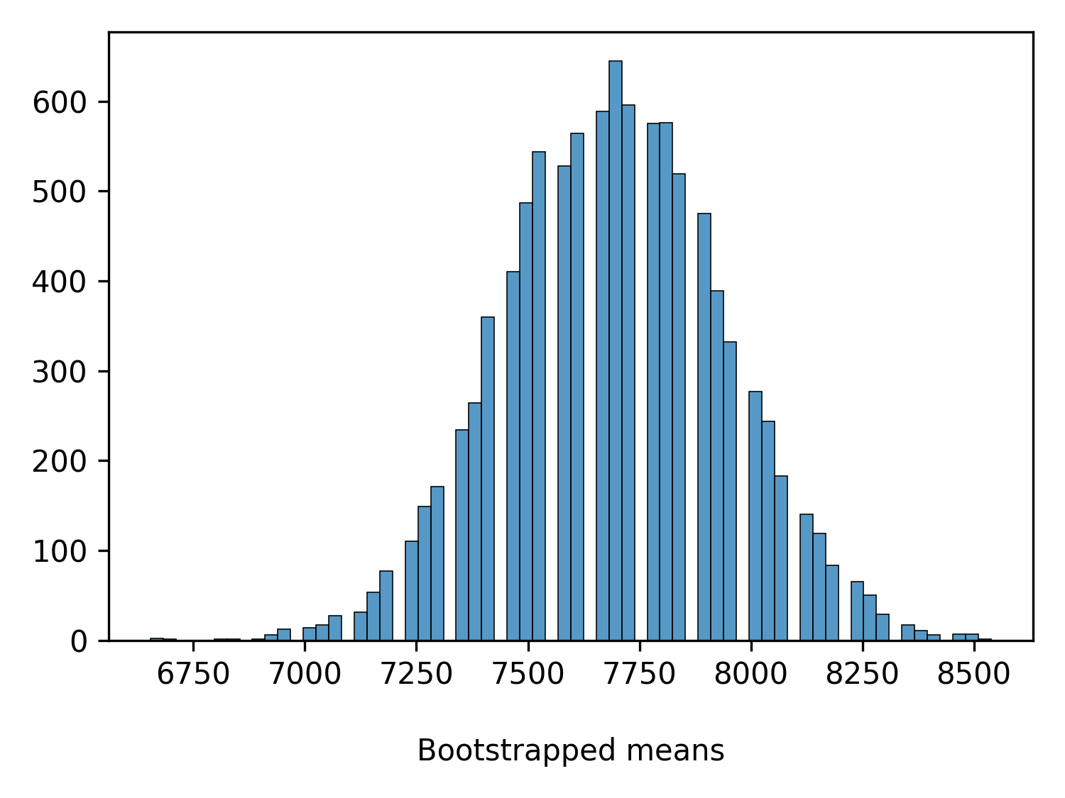
Boot = stats.bootstrap(Steps, np.mean, confidence_level=0.95, method='BCa')
print(Boot.confidence_interval)
ConfidenceInterval(low=7192.307692307692, high=8153.846153846154)
round(Boot.confidence_interval[0], 0)
7192.0
round(Boot.confidence_interval[1], 0)
8192.0
### Note that results by bootstrap may vary
plt.figure(figsize=(5, 3.75))
sns.histplot(x=Boot.bootstrap_distribution)
plt.title('')
plt.xlabel('\nBootstrapped means')
plt.ylabel('')
plt.grid(False)
plt.tight_layout()
plt.savefig('StepsRatingPlot.png', format='png', dpi=300)
plt.show()
Using pingouin
Steps = np.array(Data['Steps'])
stat = np.mean(Steps)
ci = pg.compute_bootci(Steps, func='mean', decimals=0)
print(round(stat, 0), ci)
7692.0 [7192. 8115.]
### Note that results by bootstrap may vary
One-way data – traditional method
Using researchpy.rp
rp.summary_cont(Data.groupby(Data['Gender'])['Steps'], conf = 0.95, decimals = 0)
N Mean SD SE 95% Conf. Interval
Gender
female 15 8200.0 1207.0 312.0 7532.0 8868.0
male 11 7000.0 1095.0 330.0 6264.0 7736.0
Two-way data – traditional method
Using researchpy.rp
rp.summary_cont(Data.groupby(['Teacher', 'Gender'])['Steps'], conf = 0.95, decimals = 0)
N Mean SD SE 95% Conf. Interval
Teacher Gender
Catbus female 6 8000.0 1414.0 577.0 6516.0 9484.0
male 4 7000.0 1633.0 816.0 4402.0 9598.0
Satsuki female 4 8500.0 577.0 289.0 7581.0 9419.0
male 3 7000.0 1000.0 577.0 4516.0 9484.0
Totoro female 5 8200.0 1483.0 663.0 6358.0 10042.0
male 4 7000.0 816.0 408.0 5701.0 8299.0
One-way data – bootstrap method
At the time of writing, I don’t know how to pass groupby results to the bootstrap function. However, the groups can be extracted manually and passed to the bootstrap function.