A Python Companion to Extension Program Evaluation

Salvatore S. Mangiafico

Kruskal–Wallis Test

Kruskal–Wallis test in SAEPER

 

For a discussion of this test, see the corresponding chapter in Summary and Analysis of Extension Program Evaluation in R (rcompanion.org/handbook/F_08.html).

 

Specific topics that may be of interest there include:

 

•  Schwenk dice and pairwise Wilcoxon–Mann–Whitney tests

 

Importing packages in this chapter

 

The following commands will import required packages used in this chapter from libraries and assign them common aliases.  You may need install these libraries first.

 

import io

 

import os

 

import numpy as np

 

import scipy.stats as stats

 

import pandas as pd

 

import pingouin as pg

 

import scikit_posthocs as sp

 

import matplotlib.pyplot as plt

 

import seaborn as sns

 

 

Setting your working directory

 

You may wish to set your working directory for exported plots.

 

os.chdir("C:/Users/Sal Mangiafico/Desktop")

 

print(os.getcwd())

 

 

Example of Kruskal–Wallis test

 

Data = pd.read_table(sep="\\s+", filepath_or_buffer=io.StringIO("""

 

 Speaker  Likert

 Pooh      3

 Pooh      5

 Pooh      4

 Pooh      4

 Pooh      4

 Pooh      4

 Pooh      4

 Pooh      4

 Pooh      5

 Pooh      5

 Piglet    2

 Piglet    4

 Piglet    2

 Piglet    2

 Piglet    1

 Piglet    2

 Piglet    3

 Piglet    2

 Piglet    2

 Piglet    3

 Tigger    4

 Tigger    4

 Tigger    4

 Tigger    4

 Tigger    5

 Tigger    3

 Tigger    5

 Tigger    4

 Tigger    4

 Tigger    3
"""))

 

### Convert Speaker to category type

 

Data['Speaker']  = Data['Speaker'].astype('category')

 

 

### Create new variable, Likert.f as a category variable

 

Data['Likert.f']  = Data['Likert'].astype('category')

 

 

### Order Speaker by desired values

 

SpeakerLevels = ['Pooh', 'Piglet', 'Tigger']

 

Data['Speaker'] = Data['Speaker'].cat.reorder_categories(SpeakerLevels)

 

 

print(Data['Speaker'].cat.categories)

 

Index(['Pooh', 'Piglet', 'Tigger'], dtype='object')

 

 

print(Data.info())

 

#   Column    Non-Null Count  Dtype  

---  ------    --------------  -----  

 0   Speaker   30 non-null     category

 1   Likert    30 non-null     int64  

 2   Likert.f  30 non-null     category

 

 

Summarize data treating Likert scores as categories

 

pd.crosstab(Data['Speaker'], Data['Likert.f'])

 

Likert.f  1  2  3  4  5

Speaker               

Pooh      0  0  1  6  3

Piglet    1  6  2  1  0

Tigger    0  0  2  6  2

 

### Counts of observations for each Speaker and Likert level.

 

 

pd.crosstab(Data['Speaker'], Data['Likert.f'], normalize='index')

 

Likert.f    1    2    3    4    5

Speaker                         

Pooh      0.0  0.0  0.1  0.6  0.3

Piglet    0.1  0.6  0.2  0.1  0.0

Tigger    0.0  0.0  0.2  0.6  0.2

 

### Note proportions add to 1.0 in each row

 

 

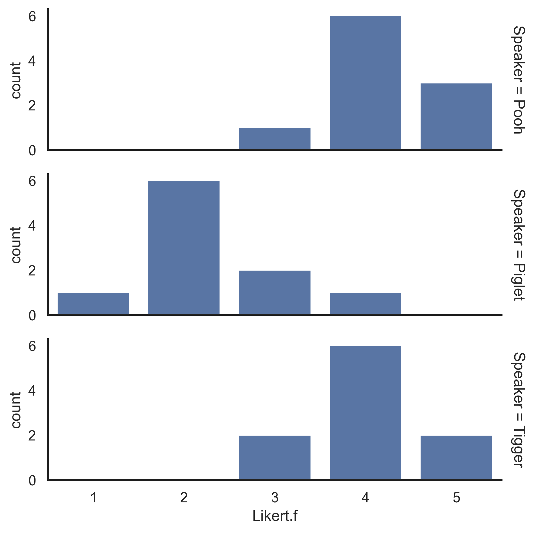
Bar plots of data by group

 

sns.set_theme(style='white')

 

Plot = sns.FacetGrid(data=Data, row='Speaker',

 

                  margin_titles=True, height=2, aspect= 3)

 

Plot.map(sns.countplot, 'Likert.f')

 

Plot.tight_layout()

 

Plot.savefig('LikertBar.png', format='png', dpi=300)

 

 

 

Summarize data treating Likert scores as numeric

 

Summary = Data.groupby('Speaker')['Likert'].describe()

 

print(Summary)

 

         count  mean       std  min  25%  50%   75%  max

Speaker                                                

Pooh      10.0   4.2  0.632456  3.0  4.0  4.0  4.75  5.0

Piglet    10.0   2.3  0.823273  1.0  2.0  2.0  2.75  4.0

Tigger    10.0   4.0  0.666667  3.0  4.0  4.0  4.00  5.0

 

 

Kruskal–Wallis test example

 

Using pingouin

 

pg.kruskal(data=Data, dv='Likert', between='Speaker')

 

          Source  ddof1          H    p-unc

Kruskal  Speaker      2  16.842308  0.00022

 

 

Using pysci.stats

 

Pooh   = np.array(Data['Likert'][Data['Speaker']== 'Pooh'])

Piglet = np.array(Data['Likert'][Data['Speaker']== 'Piglet'])

Tigger = np.array(Data['Likert'][Data['Speaker']== 'Tigger'])

 

stats.kruskal(Pooh, Piglet, Tigger)

 

KruskalResult(statistic=16.84230769230768, pvalue=0.00022016047490004256)

 

 

Effect size statistics

 

A common effect size statistic for the Kruskal–Wallis test is called epsilon-squared.  It is the same as the eta-squared (or r-squared) from a one-way analysis of variance (ANOVA) performed on the ranks on dependent variable.

 

We’ll first have to create a new variable in our data frame for the ranks of the Likert variable.

 

Data['Likert.rank'] = Data['Likert'].rank()

 

pg.anova(data=Data, dv='Likert.rank', between='Speaker', effsize='n2')

 

    Source  ddof1  ddof2          F     p-unc        n2

0  Speaker      2     27  18.701835  0.000008  0.580769

 

### Rank epsilon-squared = 0.5808

 

 

Another common effect size statistic for the Kruskal–Wallis test is called eta-squared.  Confusingly, this corresponds to the adjusted r-squared, or epsilon-squared, from an ANOVA on the ranked values.

 

Here, we’ll manually adjust the r-squared value we got above, using the sample size and number of terms in model.  Because there are three groups in the independent variable, K = 2, because there would be two dummy variables to account for those three groups in a general linear model.

 

N = len(Data['Likert'])

 

K = 2

 

RankEpsilonSq = 0.580769

 

RankEtaSq = 1 - (1 - RankEpsilonSq) * ((N - 1) / (N - K - 1))

 

round(RankEtaSq, 4)

 

0.5497

 

### Rank eta-squared = 0.5497

 

 

Post-hoc tests for multiple comparisons of groups

 

Some results below differ slightly from those reported by R.  This may have to do with differences p-value adjustment methods.

 

Dunn test

 

Several different p-value adjustment methods are available. See the function documentation for the options.

 

sp.posthoc_dunn(Data, val_col='Likert', group_col='Speaker', p_adjust='holm')

 

            Pooh    Piglet    Tigger

Pooh    1.000000  0.000489  0.630298

Piglet  0.000489  1.000000  0.002011

Tigger  0.630298  0.002011  1.0000000

 

 

Conover test

 

Several different p-value adjustment methods are available. See the function documentation for the options.

 

sp.posthoc_conover(Data, val_col='Likert', group_col='Speaker', p_adjust='sidak')

 

            Pooh    Piglet    Tigger

Pooh    1.000000  0.000017  0.858881

Piglet  0.000017  1.000000  0.000119

Tigger  0.858881  0.000119  1.000000

 

 

Nemenyi test

 

sp.posthoc_nemenyi(Data, val_col='Likert', group_col='Speaker')

 

            Pooh    Piglet    Tigger

Pooh    1.000000  0.000819  0.890628

Piglet  0.000819  1.000000  0.004478

Tigger  0.890628  0.004478  1.000000

 

 

Dwass–Steel–Critchlow–Fligner test

 

sp.posthoc_dscf(Data, val_col='Likert', group_col='Speaker')

 

            Pooh    Piglet    Tigger

Pooh    1.000000  0.001183  0.769015

Piglet  0.001183  1.000000  0.002073

Tigger  0.769015  0.002073  1.000000

 

 

Plot of medians and confidence intervals

 

The following plots the median Likert score for each Speaker, with confidence intervals for the medians, calculated with bootstrap.

 

Simple seaborn call

 

sns.catplot(data=Data, x='Speaker', y='Likert', kind='point',

            errorbar=('ci'), estimator='median', capsize=0.12,

            linestyles='none')

 

 

Formatting and export as file

 

sns.set_theme(style='darkgrid')

 

Plot = sns.catplot(data=Data, x='Speaker', y='Likert', kind='point',

            errorbar=('ci'), estimator='median', capsize=0.12,

            linestyles='none',

            height=4, aspect=1.33)

 

Plot.set_titles('')

Plot.set_xlabels('\nSpeaker')

Plot.set_ylabels('Median Likert\n')

 

Plot.tight_layout()

 

plt.text(x= -0.05, y=5.25, s="a", fontsize=12, color='black')

plt.text(x=  0.95, y=3.25, s="b", fontsize=12, color='black')

plt.text(x=  1.98, y=4.75, s="a", fontsize=12, color='black')

 

Plot.savefig('LikertMedianSpeaker.png', format='png', dpi=300)

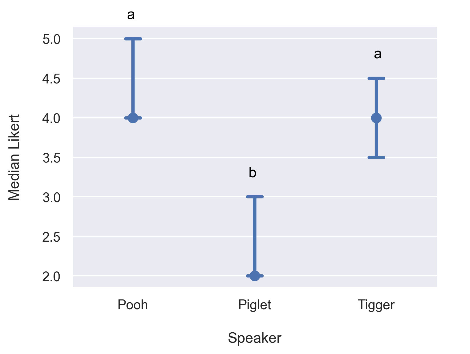
Plot of median Likert score versus Speaker.  Error bars indicate the 95% confidence intervals for the median by bootstrap method.

©2025 by Salvatore S. Mangiafico.
Rutgers Cooperative Extension, New Brunswick, NJ.

Non-commercial reproduction of this content, with attribution, is permitted.
For-profit reproduction without permission is prohibited.

If you use the code or information in this site in a published work, please cite it as a source.  Also, if you are an instructor and use this book in your course, please let me know.   My contact information is on the Author of this Book page.

Citation

Mangiafico, S.S. 2025. Summary and Analysis of Extension Program Evaluation in R, version 0.2.7, revised 2025. rcompanion.org/python/. (Pdf version: rcompanion.org/documents/PythonCompanionProgramEvaluation.pdf.)