![[banner]](images/banner.png "Batsto Lake, Wharton State Forest, New Jersey")
Examples in Summary and Analysis of Extension Program Evaluation
Packages used in this chapter
The following commands will install these packages if they are not already installed:
if(!require(FSA)){install.packages("FSA")}
if(!require(DescTools)){install.packages("DescTools")}
if(!require(rcompanion)){install.packages("rcompanion")}
if(!require(multcompView)){install.packages("multcompView")}
if(!require(PMCMRplus)){install.packages("PMCMRplus ")}
When to use it
See the Handbook for information on this topic.
Null hypothesis
This example shows just summary statistics, histograms by group, and the Kruskal–Wallis test. An example with plots, post-hoc tests, and alternative tests is shown in the “Example” section below.
Kruskal–Wallis test example
### --------------------------------------------------------------
### Kruskal–Wallis test, hypothetical example, p. 159
### --------------------------------------------------------------
Data = read.table(header=TRUE, stringsAsFactors=TRUE, text="
Group Value
Group.1 1
Group.1 2
Group.1 3
Group.1 4
Group.1 5
Group.1 6
Group.1 7
Group.1 8
Group.1 9
Group.1 46
Group.1 47
Group.1 48
Group.1 49
Group.1 50
Group.1 51
Group.1 52
Group.1 53
Group.1 342
Group.2 10
Group.2 11
Group.2 12
Group.2 13
Group.2 14
Group.2 15
Group.2 16
Group.2 17
Group.2 18
Group.2 37
Group.2 58
Group.2 59
Group.2 60
Group.2 61
Group.2 62
Group.2 63
Group.2 64
Group.2 193
Group.3 19
Group.3 20
Group.3 21
Group.3 22
Group.3 23
Group.3 24
Group.3 25
Group.3 26
Group.3 27
Group.3 28
Group.3 65
Group.3 66
Group.3 67
Group.3 68
Group.3 69
Group.3 70
Group.3 71
Group.3 72
")
### Specify the order of factor levels
## otherwise R will alphabetize them
Data$Group = factor(Data$Group, levels=unique(Data$Group))
### Examine data frame
str(Data)
Medians and descriptive statistics
As noted in the Handbook, each group has identical medians and means.
library(FSA)
Summarize(Value ~ Group,
data = Data)
Group n mean sd min Q1 median Q3 max
1 Group.1 18 43.5 77.77513 1 5.25 27.5 49.75 342
2 Group.2 18 43.5 43.69446 10 14.25 27.5 60.75 193
3 Group.3 18 43.5 23.16755 19 23.25 27.5 67.75 72
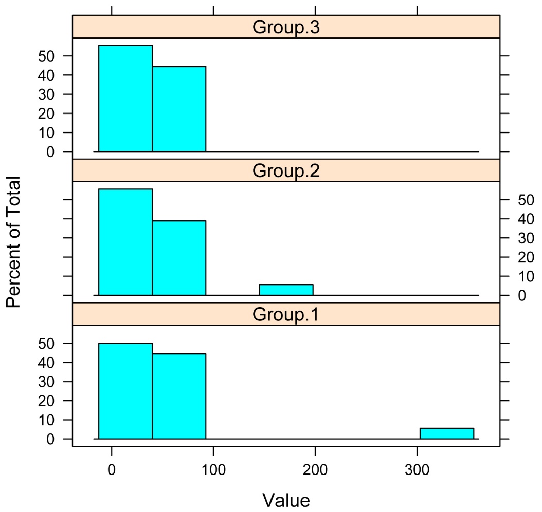
Histograms for each group
library(lattice)
histogram(~ Value | Group,
data=Data,
layout=c(1,3)) # columns and rows
of individual plots
Kruskal–Wallis test
In this case, there is a significant difference in the distributions of values among groups, as is evident both from the histograms and from the significant Kruskal–Wallis test. Only in cases where the distributions in each group are similar in shape and spread can a significant Kruskal–Wallis test be interpreted as a difference in medians.
kruskal.test(Value ~ Group,
data = Data)
Kruskal-Wallis chi-squared = 7.3553, df = 2, p-value = 0.02528
How the test works
Assumptions
See the Handbook
for information on these topics.
Example
The Kruskal–Wallis test is performed on a data frame with the kruskal.test
function in the native stats package. Shown is a complete example with
plots and post-hoc tests.
The example is data measuring if the mucociliary efficiency in the rate of dust removal is different among normal subjects, subjects with obstructive airway disease, and subjects with asbestosis. For the original citation, use the ?kruskal.test command.
For both the submissive dog example and the oyster DNA example from the Handbook, a Kruskal–Wallis test is shown later in this chapter.
Kruskal–Wallis test example
###
--------------------------------------------------------------
### Kruskal–Wallis test, asbestosis example from R help for
### kruskal.test
### --------------------------------------------------------------
Data = read.table(header=TRUE, stringsAsFactors=TRUE, text="
Obs Health Efficiency
1 Normal 2.9
2 Normal 3.0
3 Normal 2.5
4 Normal 2.6
5 Normal 3.2
6 OAD 3.8
7 OAD 2.7
8 OAD 4.0
9 OAD 2.4
10 Asbestosis 2.8
11 Asbestosis 3.4
12 Asbestosis 3.7
13 Asbestosis 2.2
14 Asbestosis 2.0
")
### Specify the order of factor levels
## otherwise R will alphabetize them
Data$Health = factor(Data$Health, levels=unique(Data$Health))
Medians and descriptive statistics
library(FSA)
Summarize(Efficiency ~ Health,
data = Data)
Health n mean sd min Q1 median Q3 max
1 Normal 5 2.840 0.2880972 2.5 2.600 2.90 3.00 3.2
2 OAD 4 3.225 0.7932003 2.4 2.625 3.25 3.85 4.0
3 Asbestosis 5 2.820 0.7362065 2.0 2.200 2.80 3.40 3.7
Graphing the results
Stacked histograms of values across groups
library(lattice)
histogram(~ Efficiency | Health,
data=Data,
layout=c(1,3)) # columns and rows
of individual plots

Simple box plots of values across groups
boxplot(Efficiency ~ Health,
data = Data,
ylab="Efficiency",
xlab="Health")

Kruskal–Wallis test
kruskal.test(Efficiency ~ Health,
data = Data)
Kruskal-Wallis chi-squared = 0.7714, df = 2, p-value = 0.68
Dunn test for multiple comparisons
If the Kruskal–Wallis test is significant, a post-hoc
analysis can be performed to determine which levels of the independent variable
differ from each other level. Probably the most popular test for this is the
Dunn test, which is performed with the dunnTest function in the FSA
package. Adjustments to the p-values could be made using the method
option to control the familywise error rate or to control the false discovery
rate. See ?p.adjust for details.
Zar (2010) states that the Dunn test is appropriate for groups with unequal
numbers of observations.
If there are several values to compare, it can be beneficial to have R convert
this table to a compact letter display for you. The cldList function in
the rcompanion package can do this.
### Order groups by median
Data$Health = factor(Data$Health,
levels=c("OAD", "Normal",
"Asbestosis"))
### Dunn test
library(FSA)
PT = dunnTest(Efficiency ~ Health,
data=Data,
method="bh") # Can
adjust p-values;
# See ?p.adjust for options
PT
Dunn (1964) Kruskal-Wallis multiple comparison
p-values adjusted with the Benjamini-Hochberg method.
Comparison Z P.unadj P.adj
1 Asbestosis - Normal -0.2267787 0.8205958 0.8205958
2 Asbestosis - OAD -0.8552360 0.3924205 1.0000000
3 Normal - OAD -0.6414270 0.5212453 0.7818680
PTD = PT$res
library(rcompanion)
cldList(comparison = PTD$Comparison,
p.value = PTD$P.adj,
threshold = 0.05)
Group Letter MonoLetter
1 Asbestosis a a
2 Normal a a
3 OAD a a
### Values sharing the same letter are not
significantly different
Nemenyi test for multiple comparisons
Zar (2010) suggests that the Nemenyi test is not appropriate for groups with unequal numbers of observations.
library(DescTools)
PT = NemenyiTest(x = Data$Efficiency,
g = Data$Health,
dist="tukey")
PT
Nemenyi's test of multiple comparisons for independent samples
(tukey)
mean.rank.diff pval
Normal-OAD -1.8 0.7972
Asbestosis-OAD -2.4 0.6686
Asbestosis-Normal -0.6 0.9720
PTD = as.data.frame(PT[1])
library(rcompanion)
cldList(comparison = row.names(PTD,
p.value = PTD$pval,
threshold = 0.05)
Group Letter MonoLetter
1 Normal a a
2 Asbestosis a a
3 OAD a a
### Values sharing the same letter are not
significantly different
Kruskal–Wallis test example
###
--------------------------------------------------------------
### Kruskal–Wallis test, submissive dog example, pp. 161–162
### --------------------------------------------------------------
Data = read.table(header=TRUE, stringsAsFactors=TRUE, text="
Dog Sex Rank
Merlino Male 1
Gastone Male 2
Pippo Male 3
Leon Male 4
Golia Male 5
Lancillotto Male 6
Mamy Female 7
Nanà Female 8
Isotta Female 9
Diana Female 10
Simba Male 11
Pongo Male 12
Semola Male 13
Kimba Male 14
Morgana Female 15
Stella Female 16
Hansel Male 17
Cucciola Male 18
Mammolo Male 19
Dotto Male 20
Gongolo Male 21
Gretel Female 22
Brontolo Female 23
Eolo Female 24
Mag Female 25
Emy Female 26
Pisola Female 27
")
### Specify the order of factor levels
## otherwise R will alphabetize them
Data$Sex = factor(Data$Sex, levels=unique(Data$Sex))
### Examine data frame
str(Data)
### Summarize data
library(FSA)
Summarize(Rank ~ Sex,
data = Data)
Sex n mean sd min Q1 median Q3 max
1 Male 15 11.06667 7.065678 1 4.50 12 17.50 21
2 Female 12 17.66667 7.679173 7 9.75 19 24.25 27
### Kruskal-Wallis test
kruskal.test(Rank ~ Sex,
data = Data)
Kruskal-Wallis chi-squared = 4.6095, df = 1, p-value = 0.03179
### Dunn test with PMCMRplus package
library(PMCMRplus)
DT = kwAllPairsDunnTest(Rank ~ Sex, data=Data, method="bh")
library(rcompanion)
DTT =PMCMRTable(DT)
DTT
Comparison p.value
1 Female - Male = 0 0.0318
cldList(p.value ~ Comparison, data=DTT)
Group Letter MonoLetter
1 Female a a
2 Male b b
Graphing the results
Graphing of the results is shown above in the “Example” section.
Similar tests
One-way anova is presented elsewhere in this book.
How to do the test
Kruskal–Wallis test example
### --------------------------------------------------------------
### Kruskal–Wallis test, oyster DNA example, pp. 163–164
### --------------------------------------------------------------
Data = read.table(header=TRUE, stringsAsFactor=TRUE, text="
Markername Markertype fst
CVB1 DNA -0.005
CVB2m DNA 0.116
CVJ5 DNA -0.006
CVJ6 DNA 0.095
CVL1 DNA 0.053
CVL3 DNA 0.003
6Pgd protein -0.005
Aat-2 protein 0.016
Acp-3 protein 0.041
Adk-1 protein 0.016
Ap-1 protein 0.066
Est-1 protein 0.163
Est-3 protein 0.004
Lap-1 protein 0.049
Lap-2 protein 0.006
Mpi-2 protein 0.058
Pgi protein -0.002
Pgm-1 protein 0.015
Pgm-2 protein 0.044
Sdh protein 0.024
")
### Specify the order of factor levels
## otherwise R will alphabetize them
Data$Markertype = factor(Data$ Markertype, levels=unique(Data$ Markertype))
### Examine data frame
str(Data)
### Summarize data
library(FSA)
Summarize(fst ~ Markertype,
data = Data)
Markertype n mean sd min Q1 median Q3 max
1 DNA 6 0.0426667 0.0537352 -0.006 -0.00300 0.028 0.08450 0.116
2 protein 14 0.0353571 0.0431448 -0.005 0.00825 0.020 0.04775 0.163
kruskal.test(fst ~ Markertype,
data = Data)
Kruskal-Wallis chi-squared = 0.0426, df = 1, p-value = 0.8365
Power Analysis
See the Handbook for information on this topic.
References
Zar, J.H. 2010. Biostatistical Analysis, 5th ed. Pearson Prentice Hall: Upper Saddle River, NJ.