![[banner]](images/banner.png "Batsto Lake, Wharton State Forest, New Jersey")
Examples in Summary and Analysis of Extension Program Evaluation
SAEPER: Using Random
Effects in Models
SAEPER: What are
Least Square Means?
SAEPER: One-way
ANOVA with Random Blocks
Packages used in this chapter
The following commands will install these packages if they are not already installed:
if(!require(nlme)){install.packages("nlme")}
if(!require(multcomp)){install.packages("multcomp")}
if(!require(multcompView)){install.packages("multcompView")}
if(!require(lsmeans)){install.packages("lsmeans")}
if(!require(lme4)){install.packages("lme4")}
if(!require(lmerTest)){install.packages("lmerTest")}
if(!require(TukeyC)){install.packages("TukeyC")}
When to use it
Null hypotheses
How the test works
Partitioning variance and optimal allocation of resources
Unequal sample sizes
Assumptions
Example
Graphing the results
Similar tests
See the Handbook for information on these topics.
How to do the test
Nested anova example with mixed effects model (nlme)
One approach to fit a nested anova is to use a mixed effects model. Here Tech is being treated as a fixed effect, while Rat is treated as a random effect. Note that the F-value and p-value for the test on Tech agree with the values in the Handbook. The effect of Rat will be tested by comparing this model to a model without the Rat term. The model is fit using the lme function in nlme.
### --------------------------------------------------------------
### Nested anova, SAS example, pp. 171-173
### --------------------------------------------------------------
Input =("
Tech Rat Protein
Janet 1 1.119
Janet 1 1.2996
Janet 1 1.5407
Janet 1 1.5084
Janet 1 1.6181
Janet 1 1.5962
Janet 1 1.2617
Janet 1 1.2288
Janet 1 1.3471
Janet 1 1.0206
Janet 2 1.045
Janet 2 1.1418
Janet 2 1.2569
Janet 2 0.6191
Janet 2 1.4823
Janet 2 0.8991
Janet 2 0.8365
Janet 2 1.2898
Janet 2 1.1821
Janet 2 0.9177
Janet 3 0.9873
Janet 3 0.9873
Janet 3 0.8714
Janet 3 0.9452
Janet 3 1.1186
Janet 3 1.2909
Janet 3 1.1502
Janet 3 1.1635
Janet 3 1.151
Janet 3 0.9367
Brad 5 1.3883
Brad 5 1.104
Brad 5 1.1581
Brad 5 1.319
Brad 5 1.1803
Brad 5 0.8738
Brad 5 1.387
Brad 5 1.301
Brad 5 1.3925
Brad 5 1.0832
Brad 6 1.3952
Brad 6 0.9714
Brad 6 1.3972
Brad 6 1.5369
Brad 6 1.3727
Brad 6 1.2909
Brad 6 1.1874
Brad 6 1.1374
Brad 6 1.0647
Brad 6 0.9486
Brad 7 1.2574
Brad 7 1.0295
Brad 7 1.1941
Brad 7 1.0759
Brad 7 1.3249
Brad 7 0.9494
Brad 7 1.1041
Brad 7 1.1575
Brad 7 1.294
Brad 7 1.4543
")
Data = read.table(textConnection(Input),header=TRUE)
### Since Rat is read in as an integer variable,
convert it to factor
Data$Rat = as.factor(Data$Rat)
library(nlme)
model = lme(Protein ~ Tech, random=~1|Rat,
data=Data,
method="REML")
anova.lme(model,
type="sequential",
adjustSigma = FALSE)
numDF denDF F-value p-value
(Intercept) 1 54 587.8664 <.0001
Tech 1 4 0.2677 0.6322
Post-hoc comparison of means
Note that “Tukey” here instructs the glht function to compare all means, not to perform a Tukey adjustment of multiple comparisons.
library(multcomp)
posthoc = glht(model,
linfct = mcp(Tech="Tukey"))
mcs = summary(posthoc,
test=adjusted("single-step"))
mcs
### Adjustment options: "none",
"single-step", "Shaffer",
### "Westfall", "free",
"holm", "hochberg",
### "hommel", "bonferroni",
"BH", "BY", "fdr"
Linear Hypotheses:
Estimate Std. Error z value Pr(>|z|)
Janet - Brad == 0 -0.05060 0.09781 -0.517 0.605
cld(mcs,
level=0.05,
decreasing=TRUE)
Brad Janet
"a" "a"
### Means sharing a letter are not
significantly different
Post-hoc comparison of least-square means
Least squares means are adjusted for other terms in the
model. If the experimental design is unbalanced or there is missing data, the
least square means may differ significantly from arithmetic means for
treatments, but are generally more representative of the population means than
the arithmetic means would be.
Note that the adjustments for multiple comparisons (adjust =”tukey”) appears in
both the lsmeans and cld functions.
library(multcompView)
library(lsmeans)
leastsquare = lsmeans(model,
pairwise ~ Tech,
adjust="tukey") ###
Tukey-adjusted comparisons
leastsquare
$lsmeans
Tech lsmean SE df lower.CL upper.CL
Brad 1.211023 0.06916055 5 1.0332405 1.388806
Janet 1.160420 0.06916055 4 0.9683995 1.352440
Confidence level used: 0.95
$contrasts
contrast estimate SE df t.ratio p.value
Brad - Janet 0.05060333 0.09780778 4 0.517 0.6322
cld(leastsquare,
alpha=0.05,
Letters=letters, ### Use lower-case
letters for .group
adjust="tukey") ###
Tukey-adjusted comparisons
Tech lsmean SE df asymp.LCL asymp.UCL .group
Janet 1.160420 0.06916018 NA 1.005745 1.315095 a
Brad 1.211023 0.06916018 NA 1.056348 1.365698 a
### Means sharing a letter in .group are not
significantly different
Test the significance of the random effect in the mixed effects model
In order to the test the significance of the random effect from our model (Rat), we can fit a new model with only the fixed effects from the model. For this we use the gls function in the nlme package. We then compare the two models with the anova fuction. Note that the p-value does not agree with p-value from the Handbook, because the technique is different, though in this case the conclusion is the same. As a general precaution, if your models are fit with “REML” (restricted maximum likelihood) estimation, then you should compare only models with the same fixed effects. If you need to compare models with different fixed effects, use “ML” as the estimation method for all models.
model.fixed = gls(Protein ~ Tech,
data=Data,
method="REML")
anova(model,
model.fixed)
Model df AIC BIC logLik Test L.Ratio p-value
model 1 4 -7.819054 0.4227176 7.909527
model.fixed 2 3 -4.499342 1.6819872 5.249671 1 vs 2 5.319713 0.0211
Checking assumptions of the model
hist(residuals(model),
col="darkgray")
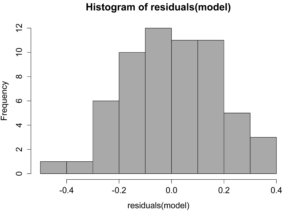
A histogram of residuals from a linear model. The distribution of these residuals should be approximately normal.
plot(fitted(model),
residuals(model))
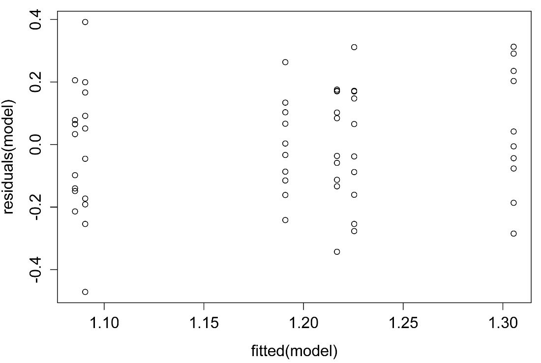
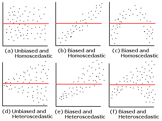
A plot of residuals vs. predicted values. The residuals should be unbiased and homoscedastic. For an illustration of these properties, see this diagram by Steve Jost at DePaul University: condor.depaul.edu/sjost/it223/documents/resid-plots.gif.
### additional model checking plots with: plot(model)
Mixed effects model with lmer
The following is an abbreviated example of a nested anova using the lmer function in the lme4 package. See the previous example in this chapter for explanation and model-checking.
###
--------------------------------------------------------------
### Nested anova, SAS example, pp. 171-173
### --------------------------------------------------------------
Input =("
Tech Rat Protein
Janet 1 1.119
Janet 1 1.2996
Janet 1 1.5407
Janet 1 1.5084
Janet 1 1.6181
Janet 1 1.5962
Janet 1 1.2617
Janet 1 1.2288
Janet 1 1.3471
Janet 1 1.0206
Janet 2 1.045
Janet 2 1.1418
Janet 2 1.2569
Janet 2 0.6191
Janet 2 1.4823
Janet 2 0.8991
Janet 2 0.8365
Janet 2 1.2898
Janet 2 1.1821
Janet 2 0.9177
Janet 3 0.9873
Janet 3 0.9873
Janet 3 0.8714
Janet 3 0.9452
Janet 3 1.1186
Janet 3 1.2909
Janet 3 1.1502
Janet 3 1.1635
Janet 3 1.151
Janet 3 0.9367
Brad 5 1.3883
Brad 5 1.104
Brad 5 1.1581
Brad 5 1.319
Brad 5 1.1803
Brad 5 0.8738
Brad 5 1.387
Brad 5 1.301
Brad 5 1.3925
Brad 5 1.0832
Brad 6 1.3952
Brad 6 0.9714
Brad 6 1.3972
Brad 6 1.5369
Brad 6 1.3727
Brad 6 1.2909
Brad 6 1.1874
Brad 6 1.1374
Brad 6 1.0647
Brad 6 0.9486
Brad 7 1.2574
Brad 7 1.0295
Brad 7 1.1941
Brad 7 1.0759
Brad 7 1.3249
Brad 7 0.9494
Brad 7 1.1041
Brad 7 1.1575
Brad 7 1.294
Brad 7 1.4543
")
Data = read.table(textConnection(Input),header=TRUE)
Data$Rat = as.factor(Data$Rat)
library(lme4)
library(lmerTest)
model = lmer(Protein ~ Tech + (1|Rat),
data=Data,
REML=TRUE)
anova(model)
Analysis of Variance Table of type III with Satterthwaite
approximation for degrees of freedom
Sum Sq Mean Sq NumDF DenDF F.value Pr(>F)
Tech 0.0096465 0.0096465 1 4 0.26768 0.6322
rand(model)
Analysis of Random effects Table:
Chi.sq Chi.DF p.value
Rat 5.32 1 0.02 *
difflsmeans(model,
test.effs="Tech")
Differences of LSMEANS:
Estimate Standard Error DF t-value Lower CI Upper CI p-value
Tech Brad - Janet 0.1 0.0978 4.0 0.52 -0.221 0.322 0.6
library(multcomp)
posthoc = glht(model,
linfct = mcp(Tech="Tukey"))
mcs = summary(posthoc,
test=adjusted("single-step"))
mcs
Linear Hypotheses:
Estimate Std. Error z value Pr(>|z|)
Janet - Brad == 0 -0.05060 0.09781 -0.517 0.605
(Adjusted p values reported -- single-step method)
cld(mcs,
level=0.05,
decreasing=TRUE)
Brad Janet
"a" "a"
# # #
Nested anova example with the aov function
###
--------------------------------------------------------------
### Nested anova, SAS example, pp. 171-173
### --------------------------------------------------------------
Input =("
Tech Rat Protein
Janet 1 1.119
Janet 1 1.2996
Janet 1 1.5407
Janet 1 1.5084
Janet 1 1.6181
Janet 1 1.5962
Janet 1 1.2617
Janet 1 1.2288
Janet 1 1.3471
Janet 1 1.0206
Janet 2 1.045
Janet 2 1.1418
Janet 2 1.2569
Janet 2 0.6191
Janet 2 1.4823
Janet 2 0.8991
Janet 2 0.8365
Janet 2 1.2898
Janet 2 1.1821
Janet 2 0.9177
Janet 3 0.9873
Janet 3 0.9873
Janet 3 0.8714
Janet 3 0.9452
Janet 3 1.1186
Janet 3 1.2909
Janet 3 1.1502
Janet 3 1.1635
Janet 3 1.151
Janet 3 0.9367
Brad 5 1.3883
Brad 5 1.104
Brad 5 1.1581
Brad 5 1.319
Brad 5 1.1803
Brad 5 0.8738
Brad 5 1.387
Brad 5 1.301
Brad 5 1.3925
Brad 5 1.0832
Brad 6 1.3952
Brad 6 0.9714
Brad 6 1.3972
Brad 6 1.5369
Brad 6 1.3727
Brad 6 1.2909
Brad 6 1.1874
Brad 6 1.1374
Brad 6 1.0647
Brad 6 0.9486
Brad 7 1.2574
Brad 7 1.0295
Brad 7 1.1941
Brad 7 1.0759
Brad 7 1.3249
Brad 7 0.9494
Brad 7 1.1041
Brad 7 1.1575
Brad 7 1.294
Brad 7 1.4543
")
Data = read.table(textConnection(Input),header=TRUE)
### Since Rat is read in as an integer variable,
convert it to factor
Data$Rat = as.factor(Data$Rat)
Using the aov function for a nested anova
The aov function in the native stats package allows
you to specify an error component to the model. When formulating this model in
R, the correct error is Rat, not Tech/Rat (Rat within Tech)
as used in the SAS example. The SAS model will tolerate Rat or Rat(Tech).
The summary of the aov will produce the correct test for Tech.
The test for Rat can be performed by manually calculating the p-value
for the F-test using the output for Error:Rat and Error:Within.
See the rattlesnake example in the Two-way anova chapter for designating
an error term in a repeated-measures model.
fit = aov(Protein ~ Tech + Error(Rat), data=Data)
summary(fit)
Error: Rat
Df Sum Sq Mean Sq F value Pr(>F)
Tech 1 0.0384 0.03841 0.268 0.632
Residuals 4 0.5740 0.14349
### This matches “use for groups” in the
Handbook
Using Mean Sq and Df values to get p-value for H = Tech and Error = Rat
pf(q=0.03841/0.14349,
df1=1,
df2=4,
lower.tail=FALSE)
[1] 0.6321845
### Note: This is same test as summary(fit)
Using Mean Sq and Df values to get p-value for H = Rat and Error = Within
summary(fit)
Error: Within
Df Sum Sq Mean Sq F value Pr(>F)
Residuals 54 1.946 0.03604
pf(q=0.14349/0.03604,
df1=4,
df2=54,
lower.tail=F)
[1] 0.006663615
### Matches “use for subgroups” in the Handbook
Post-hoc comparison of means with Tukey
The aov function with an Error component produces an object of aovlist type, which unfortunately isn’t handled by many post-hoc testing functions. However, in the TukeyC package, you can specify a model and error term. For unbalanced data, the dispersion parameter may need to be modified.
library(TukeyC)
tuk = TukeyC(Data,
model = 'Protein ~ Tech + Error(Rat)',
error = 'Rat',
which = 'Tech',
fl1=1,
sig.level = 0.05)
summary(tuk)
Groups of means at sig.level = 0.05
Means G1
Brad 1.21 a
Janet 1.16 a
# # #