R Handbook: Kruskal–Wallis Test

The Kruskal–Wallis test is a rank-based test that is similar to the Mann–Whitney U test, but can be applied to one-way data with more than two groups.

Without further assumptions about the distribution of the data, the Kruskal–Wallis test does not address hypotheses about the medians of the groups. Instead, the test addresses if it is likely that an observation in one group is greater than an observation in the other. This is sometimes stated as testing if one sample has stochastic dominance compared with the other.

The test assumes that the observations are independent. That is, it is not appropriate for paired observations or repeated measures data.

It is performed with the kruskal.test function in the native stats package.

Appropriate effect size statistics include maximum Vargha and Delaney’s A, maximum Cliff’s delta, Freeman’s theta, and epsilon-squared.

Post-hoc tests

The outcome of the Kruskal–Wallis test tells you if there are differences among the groups, but doesn’t tell you which groups are different from other groups. In order to determine which groups are different from others, post-hoc testing can be conducted. Probably the most common post-hoc test for the Kruskal–Wallis test is the Dunn test (1964). Also presented are the Conover test and Nemenyi test.

Appropriate data

• One-way data

• Dependent variable is ordinal, interval, or ratio

• Independent variable is a factor with two or more levels. That is, two or more groups

• Observations between groups are independent. That is, not paired or repeated measures data

• In order to be a test of medians, the distributions of values for each group need to be of similar shape and spread. Otherwise, the test is typically a test of stochastic equality.

Hypotheses

• Null hypothesis: The groups are sampled from populations with identical distributions. Typically, that the sampled populations exhibit stochastic equality.

• Alternative hypothesis (two-sided): The groups are sampled from populations with different distributions. Typically, that one sampled population exhibits stochastic dominance.

Interpretation

Significant results can be reported as “There was a significant difference in values among groups.”

Post-hoc analysis allows you to say “There was a significant difference in values between groups A and B.”, and so on.

Other notes and alternative tests

Mood’s median test compares the medians of groups.

Aligned ranks transformation anova (ART anova) provides nonparametric analysis for a variety of designs.

For ordinal data, an alternative is to use cumulative link models, which are described later in this book.

Tests similar to Kruskal – Wallis that account for ordinal independent variables are the Jonckheere–Terpstra and Cuzick tests.

Optional technical note on hypotheses for Kruskal–Wallis test

There is a lot of conflicting information on the null and alternate hypotheses for Mann–Whitney and Kruskal–Wallis tests. Some authors will state that they test medians, usually adding an assumption that the distributions of the groups need to be of the same shape and spread. If this assumption holds, then, yes, these tests can be thought of as tests of location such as the median.

Without this assumption, these tests compare the stochastic dominance of the groups. Once a rank transformation is applied, stochastic dominance is exhibited simply by the groups with higher values.

Conover (1999) adds the following assumption:

Either the k population distribution functions are identical, or else some of the populations tend to yield larger values than other populations do.

My understanding is that these tests may yield significant results in the case of stochastic equality and different spread among groups. Conover’s assumption bypasses this difficulty by fiat. The upshot here is one should be careful interpreting these tests when there is stochastic equality and different spreads among groups.

Packages used in this chapter

The packages used in this chapter include:

• psych

• FSA

• lattice

• coin

• multcompView

• rcompanion

• PMCMRplus

The following commands will install these packages if they are not already installed:

if(!require(psych)){install.packages("psych")}
if(!require(FSA)){install.packages("FSA")}
if(!require(lattice)){install.packages("lattice")}

if(!require(coin)){install.packages("coin")}
if(!require(multcompView)){install.packages("multcompView")}
if(!require(rcompanion)){install.packages("rcompanion")}
if(!require(PMCMRplus)){install.packages("PMCMRplus")}

Kruskal–Wallis test example

This example re-visits the Pooh, Piglet, and Tigger data from the Descriptive Statistics with the likert Package chapter.

It answers the question, “Are the scores significantly different among the three speakers?”

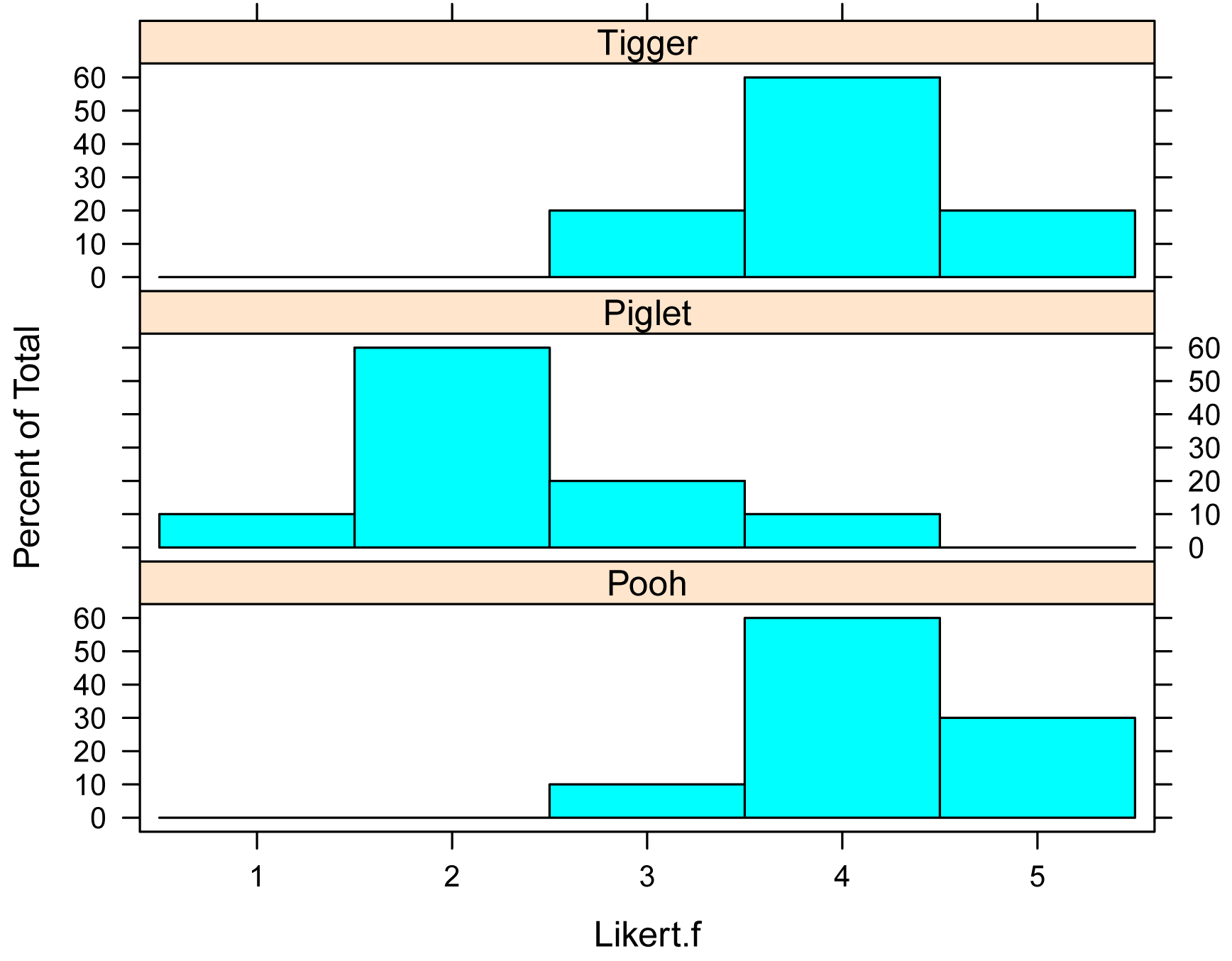
The Kruskal–Wallis test is conducted with the kruskal.test function, which produces a p-value for the hypothesis. First the data are summarized and examined using bar plots for each group.

Data = read.table(header=TRUE, stringsAsFactors=TRUE, text="

Speaker Likert
Pooh      3
Pooh      5
Pooh      4
Pooh      4
Pooh      4
Pooh     4
Pooh      4
Pooh      4
Pooh      5
Pooh      5
Piglet    2
Piglet    4
Piglet    2
Piglet    2
Piglet    1
Piglet    2
Piglet    3
Piglet    2
Piglet    2
Piglet    3
Tigger    4
Tigger    4
Tigger    4
Tigger    4
Tigger    5
Tigger    3
Tigger    5
Tigger    4
Tigger    4
Tigger    3
")

### Order levels of the factor; otherwise R will alphabetize them

Data$Speaker = factor(Data$Speaker,
                      levels=unique(Data$Speaker))

### Create a new variable which is the likert scores as an ordered factor

Data$Likert.f = factor(Data$Likert,
                       ordered = TRUE)

### Check the data frame

library(psych)

headTail(Data)

str(Data)

summary(Data)

Summarize data treating Likert scores as factors

xtabs( ~ Speaker + Likert.f,
data = Data)

Likert.f
Speaker 1 2 3 4 5
Pooh 0 0 1 6 3
Piglet 1 6 2 1 0
Tigger 0 0 2 6 2

XT = xtabs( ~ Speaker + Likert.f,
data = Data)

prop.table(XT,
margin = 1)

        Likert.f
Speaker    1   2   3   4   5
Pooh   0.0 0.0 0.1 0.6 0.3
Piglet 0.1 0.6 0.2 0.1 0.0
Tigger 0.0 0.0 0.2 0.6 0.2

Bar plots of data by group

library(lattice)

histogram(~ Likert.f | Speaker,
          data=Data,
          layout=c(1,3)      # columns and rows of individual plots
          )

Summarize data treating Likert scores as numeric

library(FSA)

Summarize(Likert ~ Speaker,
data=Data,
digits=3)

Speaker n mean    sd min Q1 median   Q3 max percZero
1    Pooh 10 4.2 0.632   3 4      4 4.75   5        0
2 Piglet 10 2.3 0.823   1 2      2 2.75   4        0
3 Tigger 10 4.0 0.667   3 4      4 4.00   5        0

Kruskal–Wallis test example

This example uses the formula notation indicating that Likert is the dependent variable and Speaker is the independent variable. The data= option indicates the data frame that contains the variables. For the meaning of other options, see ?kruskal.test.

kruskal.test(Likert ~ Speaker,
data = Data)

Kruskal-Wallis rank sum test

Kruskal-Wallis chi-squared = 16.842, df = 2, p-value = 0.0002202

As an alternative, the Kruskal–Wallis test can be conducted by Monte Carlo simulation with the coin package.

library(coin)

kruskal_test(Likert ~ Speaker, data = Data,
distribution = approximate(nresample = 10000))

Approximative Kruskal-Wallis Test

chi-squared = 16.842, p-value < 1e-04

Effect size statistics

Common effect size statistics for the Kruskal–Wallis test include epsilon-squared and eta-squared, with epsilon-squared being probably the most common. These two statistics often produce similar results. It’s important to note that both epsilon-squared and eta-squared have versions for ANOVA that are distinct from those versions for Kruskal–Wallis. It is therefore important to be sure that an appropriate implementation is chosen. Formulae for these statistics can be found in King and others (2018) and Cohen (2013), respectively.

Technical note: Interestingly, it appears that the epsilon-squared statistic for Kruskal–Wallis corresponds to the eta-squared statistic for ANOVA on ranks. However, the definitions presented here appear to be well-established.

For Freeman’s theta, an effect size of 1 indicates that the measurements for each group are entirely greater or entirely less than some other group, and an effect size of 0 indicates that there is no effect; that is, that the groups are absolutely stochastically equal.

Another option is to use the maximum Cliff’s delta or Vargha and Delaney’s A (VDA) from pairwise comparisons of all groups. VDA is the probability that an observation from one group is greater than an observation from the other group. Because of this interpretation, VDA is an effect size statistic that is relatively easy to understand.

Interpretation of effect sizes necessarily varies by discipline and the expectations of the experiment. The following guidelines are based on my personal intuition or published values. They should not be considered universal.

Technical note: The values for the interpretations for Freeman’s theta to epsilon-squared below were derived by keeping the interpretation for epsilon-squared constant and equal to that for the Mann–Whitney test. Interpretation values for Freeman’s theta were determined through comparing Freeman’s theta to epsilon-squared for simulated data (5-point Likert items, n per group between 4 and 25).

Interpretations for Vargha and Delaney’s A and Cliff’s delta come from Vargha and Delaney (2000).

	small	medium	large
epsilon-squared	0.01 – < 0.08	0.08 – < 0.26	≥ 0.26
*Freeman’s theta, k = 2*	0.11 – < 0.34	0.34 – < 0.58	≥ 0.58
*Freeman’s theta, k = 3*	0.05 – < 0.26	0.26 – < 0.46	≥ 0.46
*Freeman’s theta, k = 5*	0.05 – < 0.21	0.21 – < 0.40	≥ 0.40
*Freeman’s theta, k = 7*	0.05 – < 0.20	0.20 – < 0.38	≥ 0.38
*Freeman’s theta, k = 7*	0.05 – < 0.20	0.20 – < 0.38	≥ 0.38
Maximum Cliff’s delta	0.11 – < 0.28	0.28 – < 0.43	≥ 0.43
Maximum Vargha and Delaney’s A	0.56 – < 0.64 > 0.34 – 0.44	0.64 – < 0.71 > 0.29 – 0.34	≥ 0.71 ≤ 0.29

Ordinal epsilon-squared

library(rcompanion)

epsilonSquared(x = Data$Likert,
g = Data$Speaker)

epsilon.squared
0.581

epsilonSquared(x = Data$Likert,
g = Data$Speaker,
ci=TRUE)

### Confidence interval endpoints may vary

epsilon.squared lower.ci upper.ci
1 0.581 0.325 0.805

r-squared for anova on ranks

summary(lm(rank(Likert) ~ Speaker, data=Data))$r.squared

[1] 0.5807692

Ordinal eta-squared

library(rcompanion)

ordinalEtaSquared(x = Data$Likert,
g = Data$Speaker)

eta.squared
0.55

ordinalEtaSquared (x = Data$Likert,
g = Data$Speaker,
ci = TRUE)

eta.squared lower.ci upper.ci
1 0.55 0.293 0.794

### Confidence interval endpoints may vary

adjusted r-squared for anova on ranks

summary(lm(rank(Likert) ~ Speaker, data=Data))$adj.r.squared

[1] 0.5497151

Freeman’s theta

library(rcompanion)

freemanTheta(x = Data$Likert,
g = Data$Speaker)

Freeman.theta
0.64

freemanTheta(x = Data$Likert,
g = Data$Speaker,
ci = TRUE)

### Confidence interval endpoints may vary

Freeman.theta lower.ci upper.ci
1 0.64 0.445 0.84

Maximum Vargha and Delaney’s A or Cliff’s delta

Here, the multiVDA function is used to calculate Vargha and Delaney’s A (VDA), Cliff’s delta (CD), and the Glass rank biserial correlation coefficient (rg) between all pairs of groups. The function identifies the comparison with the most extreme VDA statistic (0.95 for Pooh – Piglet). That is, it identifies the most disparate groups.

library(rcompanion)

multiVDA(x = Data$Likert,
g = Data$Speaker)

$pairs
       Comparison VDA    CD    rg VDA.m CD.m rg.m
1   Pooh - Piglet 0.95 0.90 0.90 0.95 0.90 0.90
2   Pooh - Tigger 0.58 0.16 0.16 0.58 0.16 0.16
3 Piglet - Tigger 0.07 -0.86 -0.86 0.93 0.86 0.86

$comparison
     Comparison
"Pooh - Piglet"

$statistic
VDA
0.95

$statistic.m
VDA.m
0.95

Post-hoc test: Dunn test for multiple comparisons of groups

If the Kruskal–Wallis test is significant, a post-hoc analysis can be performed to determine which groups differ from each other group.

Probably the most popular post-hoc test for the Kruskal–Wallis test is the Dunn test. Also presented are the Conover test and Nemenyi test.

Because the post-hoc test will produce multiple p-values, adjustments to the p-values can be made to avoid inflating the possibility of making a type-I error. There are a variety of methods for controlling the familywise error rate or for controlling the false discovery rate. See ?p.adjust for details on these methods.

When there are many p-values to evaluate, it is useful to condense a table of p-values to a compact letter display format. In the output, groups are separated by letters. Groups sharing the same letter are not significantly different. Compact letter displays are a clear and succinct way to present results of multiple comparisons. However, they suffer from presenting “non-differences” instead of differences among groups, and they obscure the actual p-values, which are more informative than just a p ≤ 0.05 cutoff.

### Order groups by median

Data$Speaker = factor(Data$Speaker,
                      levels=c("Pooh", "Tigger", "Piglet"))

levels(Data$Speaker)

   ### At the time of writing, it doesn’t appear that ordering the groups affects
   ### the dunnTest output.

### Dunn test

library(FSA)

DT = dunnTest(Likert ~ Speaker,
              data=Data,
              method="bh")     # Adjusts p-values for multiple comparisons;
                                # See ?dunnTest for options

DT

Dunn (1964) Kruskal-Wallis multiple comparison
p-values adjusted with the Benjamini-Hochberg method.

       Comparison          Z      P.unadj        P.adj
1   Piglet - Pooh -3.7702412 0.0001630898 0.0004892695
2 Piglet - Tigger -3.2889338 0.0010056766 0.0015085149
3   Pooh - Tigger 0.4813074 0.6302980448 0.6302980448

### Compact letter display

PT = DT$res

PT

library(rcompanion)

cldList(P.adj ~ Comparison,
data = PT,
threshold = 0.05)

   Group Letter MonoLetter
1 Piglet      a         a
2   Pooh      b          b
3 Tigger      b          b

### Groups sharing a letter not signficantly different (alpha = 0.05).

Post-hoc tests: Dunn test, Conover test, Nemenyi test, and Dwass–Steel–Critchlow–Fligner test

### Order groups by median

Data$Speaker = factor(Data$Speaker,
levels=c("Pooh", "Tigger", "Piglet"))

levels(Data$Speaker)

Dunn test

library(PMCMRplus)

DT = kwAllPairsDunnTest(Likert ~ Speaker, data=Data, method="bh")

DT

Pairwise comparisons using Dunn's all-pairs test

Pooh Tigger
Tigger 0.63030 -
Piglet 0.00049 0.00201

P value adjustment method: holm

library(rcompanion)

DTT =PMCMRTable(DT)

DTT

           Comparison p.value
1   Tigger - Pooh = 0     0.63
2   Piglet - Pooh = 0 0.000489
3 Piglet - Tigger = 0 0.00201

cldList(p.value ~ Comparison, data=DTT)

   Group Letter MonoLetter
1 Tigger      a         a
2 Piglet      b          b
3   Pooh      a         a

Conover test

library(PMCMRplus)

CT = kwAllPairsConoverTest(Likert ~ Speaker, data=Data)

CT

Pairwise comparisons using Conover's all-pairs test

Pooh Tigger
Tigger 0.75549 -
Piglet 1.7e-05 0.00011

P value adjustment method: single-step

library(rcompanion)

CTT =PMCMRTable(CT)

CTT

           Comparison p.value
1   Tigger - Pooh = 0    0.755
2   Piglet - Pooh = 0 1.69e-05
3 Piglet - Tigger = 0 0.000115

cldList(p.value ~ Comparison, data=CTT)

   Group Letter MonoLetter
1 Tigger      a         a
2 Piglet      b         b
3   Pooh      a         a

Nemenyi test

library(PMCMRplus)

NT = kwAllPairsNemenyiTest(Likert ~ Speaker, data=Data)

NT

Pairwise comparisons using Tukey-Kramer-Nemenyi all-pairs test with Tukey-Dist approximation

Pooh Tigger
Tigger 0.8912 -
Piglet 0.0010 0.0051

P value adjustment method: single-step

library(rcompanion)

NTT =PMCMRTable(NT)

NTT

           Comparison p.value
1   Tigger - Pooh = 0    0.891
2   Piglet - Pooh = 0 0.000996
3 Piglet - Tigger = 0 0.00507

cldList(p.value ~ Comparison, data=NTT)

   Group Letter MonoLetter
1 Tigger      a         a
2 Piglet      b          b
3   Pooh      a         a

Dwass–Steel–Critchlow–Fligner test

My understanding is that the Dwass–Steel–Critchlow–Fligner test re-ranks the data with each pairwise comparison and uses a method to control the familywise error rate of multiple corrections.

library(PMCMRplus)

DSCF = dscfAllPairsTest(Likert ~ Speaker, data=Data)

DSCF

Pairwise comparisons using Dwass-Steele-Critchlow-Fligner all-pairs test

Pooh Tigger
Tigger 0.7690 -
Piglet 0.0012 0.0021

P value adjustment method: single-step

library(rcompanion)

DSCFT =PMCMRTable(DSCF)

DSCFT

#           Comparison p.value
#1   Tigger - Pooh = 0   0.769
#2   Piglet - Pooh = 0 0.00118
#3 Piglet - Tigger = 0 0.00207

cldList(p.value ~ Comparison, data=DSCFT)

#   Group Letter MonoLetter
#1 Tigger      a         a
#2 Piglet      b          b
#3   Pooh      a         a

Plot of medians and confidence intervals

The following code uses the groupwiseMedian function to produce a data frame of medians for each speaker along with the 95% confidence intervals for each median with the percentile method. These medians are then plotted, with their confidence intervals shown as error bars. The grouping letters from the multiple comparisons (Dunn test) are added.

Note that bootstrapped confidence intervals may not be reliable for discreet data, such as the ordinal Likert data used in these examples, especially for small samples.

library(rcompanion)

Sum = groupwiseMedian(Likert ~ Speaker,
                      data       = Data,
                      conf       = 0.95,
                      R          = 5000,
                      percentile = TRUE,
                      bca        = FALSE,
                      digits     = 3)

Sum

Speaker n Median Conf.level Percentile.lower Percentile.upper
1    Pooh 10      4       0.95              4.0              5.0
2 Piglet 10      2       0.95              2.0              3.0
3 Tigger 10      4       0.95              3.5              4.5

X     = 1:3
Y     = Sum$Percentile.upper + 0.2
Label = c("a", "b", "a")

library(ggplot2)

ggplot(Sum,                ### The data frame to use.
       aes(x = Speaker,
           y = Median)) +
   geom_errorbar(aes(ymin = Percentile.lower,
                     ymax = Percentile.upper),
                     width = 0.05,
                     size = 0.5) +
   geom_point(shape = 15,
              size = 4) +
   theme_bw() +
   theme(axis.title   = element_text(face = "bold")) +

   ylab("Median Likert score") +

annotate("text",
         x = X,
         y = Y,
         label = Label)

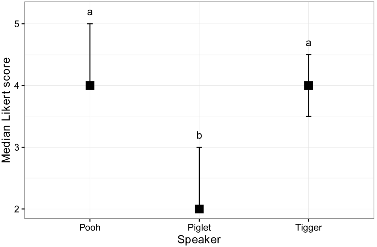
Plot of median Likert score versus Speaker. Error bars indicate the 95% confidence intervals for the median with the percentile method.

Optional technical note: Schwenk dice and pairwise Wilcoxon–Mann–Whitney tests

When choosing a post-hoc test, it is often tempting to use pairwise tests, usually with a p-value adjustment to control the familywise error rate or the false discovery rate. One issue with pairwise tests is that they ignore all the data that isn’t included in that pair of treatments. It is often better to use a post-hoc test designed to assess pairs of treatments based on the totality of the data.

In the case of the Kruskal–Wallis test, it is often desirable to use e.g. the Dunn (1964) test that preserves the rankings from all of the original data, rather than to use pairwise Mann–Whitney tests where each test would re-rank the data based only on that pair of treatments being compared.

An interesting example of the difference between these two approaches are non-transitive dice. One example is Schwenk’s dice, which are described in Futility Closet (2018) and originally by Schwenk (2000).

Imagine three six-sided dice, which have the following numbers marked on each of the sides. We want to use rank-based statistics to determine which die tends to have higher numbers.

Red = c(2,2,2,11,11,14)
Blue = c(0,3,3,12,12,12)
Green = c(1,1,1,13,13,13)

A simple way to determine which die is stochastically larger is to use Cliff’s delta.

library(rcompanion)

cliffDelta(x=Red, y=Blue)

Cliff.delta
-0.167

### The negative Cliff’s delta value suggests the values in Blue tend to be
### greater than those in Red.

### Specifically, when rolled, the Blue die beats the Red 7 / 12 times.

### ( –0.167 / 2 + 0.5 = 0.4165 = 5 / 12 )
### vda(x=Red, y=Blue) = 0.4165

cliffDelta(x=Red, y=Green)

Cliff.delta
0.167

### The positive Cliff’s delta value suggests the values in Red tend to be
### greater than those in Green.

### Specifically, when rolled, the Red die beats the Green 7 / 12 times.

cliffDelta(x=Blue, y=Green)

Cliff.delta
-0.167

### The positive Cliff’s delta value suggests the values in Green tend to be
### greater than those in Blue.

### Specifically, when rolled, the Green die beats the Blue 7 / 12 times.

So, in summary, Blue > Red, Red > Green, and Green > Blue. When viewed together, these results would be difficult to interpret, or, honestly, to make sense of.

The same could be shown with pairwise Mann–Whitney tests, if we kept the same data, but increase the sample size. I’ll refer to this new data set as representing three “groups”.

RedBig = rep(c(2,2,2,11,11,14), 25)
BlueBig = rep(c(0,3,3,12,12,12), 25)
GreenBig = rep(c(1,1,1,13,13,13), 25)

wilcox.test(RedBig, BlueBig)

W = 9375, p-value = 0.01081

wilcoxonZ(RedBig, BlueBig)

z
-2.55

### Blue > Red

wilcox.test(RedBig, GreenBig)

W = 13125, p-value = 0.01038

wilcoxonZ(RedBig, GreenBig)

z
2.56

### Red > Green

wilcox.test(BlueBig, GreenBig)

W = 9375, p-value = 0.01038

wilcoxonZ(BlueBig, GreenBig)

z
-2.56

### Green > Blue

On the other hand, because the Dunn test retains the ranking from all three groups together, it won’t find a difference among any of the groups.

Y = c(RedBig, BlueBig, GreenBig)

Group = c(rep("Red", length(RedBig)), rep("Blue", length(BlueBig)), rep("Green", length(GreenBig)))

library(FSA)

dunnTest(Y ~ Group)

Dunn (1964) Kruskal-Wallis multiple comparison
p-values adjusted with the Holm method.

    Comparison Z P.unadj P.adj
1 Blue - Green 0      1     1
2   Blue - Red 0       1     1
3 Green - Red 0       1     1

Of course, in this case, the omnibus Kruskal–Wallis test would also find no stochastic differences among the groups.

kruskal.test(Y ~ Group)

Kruskal-Wallis rank sum test

Kruskal-Wallis chi-squared = 0, df = 2, p-value = 1

References

Cohen, B.H. 2013. Explaining Psychological Statistics, 4^th. Wiley.

Cohen, J. 1988. Statistical Power Analysis for the Behavioral Sciences, 2nd Edition. Routledge.

Conover, W.J. 1999. Practical Nonparametric Statistics, 3rd. John Wiley & Sons.

Futility Closet. 2018. "Schwenk Dice". https://www.futilitycloset.com/2018/06/27/schwenk-dice/.

King, B.M., P.J. Rosopa, and E.W. Minium. 2018. Some (Almost) Assumption-Free Tests. In Statistical Reasoning in the Behavioral Sciences, 7th ed. Wiley.

Schwenk, A.J. 2000. Beware of Geeks Bearing Grifts. Math Horizons 7(4): 10–13.

Tomczak, M. and Tomczak, E. 2014. The need to report effect size estimates revisited. An overview of some recommended measures of effect size. Trends in Sports Sciences 1(21):1–25. www.tss.awf.poznan.pl/files/3_Trends_Vol21_2014__no1_20.pdf.

Vargha, A. and H.D. Delaney. A Critique and Improvement of the CL Common Language Effect Size Statistics of McGraw and Wong. 2000. Journal of Educational and Behavioral Statistics 25(2):101–132.

Exercises L

1. Considering Pooh, Piglet, and Tigger’s data,

a. What was the median score for each instructor?

b. According to the Kruskal–Wallis test, is there a statistical difference in scores among the instructors?

c. What is the value of maximum Vargha and Delaney’s A for these data?

d. How do you interpret this value? (What does it mean? And is the standard interpretation in terms of “small”, “medium”, or “large”?)

e. Looking at the post-hoc analysis, which speakers’ scores are statistically different from which others? Who had the statistically highest scores?

f. How would you summarize the results of the descriptive statistics and tests? Include practical considerations of any differences.

2. Brian, Stewie, and Meg want to assess the education level of students in their courses on creative writing for adults. They want to know the median education level for each class, and if the education level of the classes were different among instructors.

They used the following table to code his data.

Code   Abbreviation   Level

1      < HS           Less than high school
2        HS           High school
3        BA           Bachelor’s
4        MA           Master’s
5        PhD          Doctorate

The following are the course data.

Instructor        Student Education
'Brian Griffin'   a        3
'Brian Griffin'   b        2
'Brian Griffin'   c        3
'Brian Griffin'   d        3
'Brian Griffin'   e        3
'Brian Griffin'   f        3
'Brian Griffin'   g        4
'Brian Griffin'   h        5
'Brian Griffin'   i        3
'Brian Griffin'   j        4
'Brian Griffin'   k        3
'Brian Griffin'   l        2
'Stewie Griffin' m        4
'Stewie Griffin' n        5
'Stewie Griffin' o        4
'Stewie Griffin' p        4
'Stewie Griffin' q        4
'Stewie Griffin' r        4
'Stewie Griffin' s        3
'Stewie Griffin' t        5
'Stewie Griffin' u        4
'Stewie Griffin' v        4
'Stewie Griffin' w        3
'Stewie Griffin' x        2
'Meg Griffin'     y        3
'Meg Griffin'     z        4
'Meg Griffin'     aa       3
'Meg Griffin'    ab      3
'Meg Griffin'     ac       3
'Meg Griffin'     ad       2
'Meg Griffin'     ae       3
'Meg Griffin'    af      4
'Meg Griffin'     ag       2
'Meg Griffin'     ah       3
'Meg Griffin'     ai       2
'Meg Griffin'     aj       1

For each of the following, answer the question, and show the output from the analyses you used to answer the question.

a. What was the median education level for each instructor’s class? (Be sure to report the education level, not just the numeric code!)

b. According to the Kruskal–Wallis test, is there a difference in the education level of students among the instructors?