Summary and Analysis of Extension Program Evaluation in R

Salvatore S. Mangiafico

Goodness-of-Fit Tests for Nominal Variables

Goodness-of-fit tests are used to compare proportions of levels of a nominal variable to theoretical proportions.  Common goodness-of-fit tests are G-test, chi-square, and binomial or multinomial exact tests.

 

The results of chi-square tests and G-tests can be inaccurate if statistically expected cell counts are low.  I am not aware of a clear rule of thumb for goodness-of-it tests in this regard.  One option for a rule of thumb is that all statistically expected cell counts should be 5 or greater for chi-square- and G-tests.  An option for a more detailed rule of thumb is that no more than 20% of the statistically expected counts are less than 5, and that all statistically expected counts are at least 1.

 

One approach is to use exact tests, which are not bothered by low cell counts.  However, if there are not low cell counts, using G-test or chi-square test is fine.  The advantage of chi-square tests is that your audience may be more familiar with them.

 

G-tests are also called likelihood ratio tests, and “Likelihood Ratio Chi-Square” by SAS.

 

Appropriate data

•  A nominal variable with two or more levels

•  Theoretical, typical, or neutral values for the proportions for this variable are needed for comparison

•  G-test and chi-square tests may not be appropriate if there are cells with low expected counts

•  Observations are independent of one another

 

 

Hypotheses

•  Null hypothesis:  The proportions for the levels for the nominal variable are not different from the theoretical proportions.

•  Alternative hypothesis (two-sided): The proportions for the levels for the nominal variable are different from the theoretical proportions.

 

Interpretation

Significant results can be reported as “The proportions for the levels for the nominal variable were statistically different from the theoretical proportions.”

 

Packages used in this chapter

 

The packages used in this chapter include:

•  EMT

•  XNomial

•  DescTools

•  ggplot2

•  rcompanion

 

The following commands will install these packages if they are not already installed:

if(!require(EMT)){install.packages("EMT")}
if(!require(XNomial)){install.packages("XNomial")}
if(!require(DescTools)){install.packages("DescTools")}
if(!require(ggplot2)){install.packages("ggplot2")}

if(!require(rcompanion)){install.packages("rcompanion")}

 

Goodness-of-fit tests for nominal variables example

 

As part of a demographic survey of students in his environmental issues webinar series, Alucard recorded the race and ethnicity of his students.  He wants to compare the data for his class to the demographic data for Cumberland County, New Jersey as a whole

Race                Alucard’s_class   County_proportion
White               20                0.775
Black                9                0.132
American Indian      9                0.012
Asian                1                0.054
Pacific Islander     1                0.002
Two or more races    1                0.025
-----------------  ---               ------
Total               41                1.000


Ethnicity           Alucard’s_class   County_proportion
Hispanic             7                0.174
Not Hispanic        34                0.826
-----------------   ---               -----
Total               41                1.000

Exact tests for goodness-of-fit

 

Race data

If there are more than two categories, an exact multinomial test can be used.   Here, two packages are used: EMT and XNomial.  And two different approaches are used:  a direct approach and a Monte Carlo simulation.

 

Direct approach

observed    = c(20, 9, 9, 1, 1, 1)
theoretical = c(0.775, 0.132, 0.012, 0.054, 0.002, 0.025)


library(EMT)

multinomial.test(observed, theoretical)

  ### This can take a long time !

Exact Multinomial Test, distance measure: p

    Events    pObs    p.value
   1370754       0          0

library(XNomial)

xmulti(observed, theoretical)

P value (LLR) = 1.119e-09

Monte Carlo simulation

observed    = c(20, 9, 9, 1, 1, 1)
theoretical = c(0.775, 0.132, 0.012, 0.054, 0.002, 0.025)


library(EMT)

multinomial.test(observed, theoretical,
                 MonteCarlo = TRUE)

Monte Carlo Multinomial Test

    Events    pObs    p.value
   1370754       0          0

library(XNomial)

xmonte(observed, theoretical)

P value (LLR) = 0 ± 0

Ethnicity data

If there are two categories, an exact binomial test can be used.   This can be conducted in with the binom.test function in the native stats package.

###  x is the number of successes.  And n is the total number of counts.

x =  7
n = 41
theoretical = 0.174

binom.test(x, n, theoretical)

Exact binomial test

number of successes = 7, number of trials = 41, p-value = 1

Chi-square test for goodness-of-fit

 

Race data

observed    = c(20, 9, 9, 1, 1, 1)
theoretical = c(0.775, 0.132, 0.012, 0.054, 0.002, 0.025)

chisq.test(x = observed,
           p = theoretical)

Chi-squared test for given probabilities

X-squared = 164.81, df = 5, p-value < 2.2e-16

Check expected counts

Test = chisq.test(x = observed,
                  p = theoretical)

Test$expected

[1] 31.775  5.412  0.492  2.214  0.082  1.025

### Note the low expected counts: 0.492, 0.082, and 1.025,
###  suggesting the test may not be valid.

Monte Carlo simulation

chisq.test(x = observed,
           p = theoretical,
           simulate.p.value=TRUE, B=10000)

Chi-squared test for given probabilities with simulated p-value (based on 10000 replicates)

X-squared = 164.81, df = NA, p-value = 9.999e-05

Ethnicity data

###  7 and 34 are the counts for each category.  (41 total observations.)

observed    = c(7, 34)
theoretical = c(0.174, 0.826)

chisq.test(x = observed,
           p = theoretical)

Chi-squared test for given probabilities

X-squared = 0.0030472, df = 1, p-value = 0.956

Check expected counts

Test = chisq.test(x = observed,
                  p = theoretical)

Test$expected

[1]  7.134 33.866

### There are no low expected counts.

Monte Carlo simulation

chisq.test(x = observed,
           p = theoretical,
           simulate.p.value=TRUE, B=10000)

Chi-squared test for given probabilities with simulated p-value (based on 10000 replicates)

X-squared = 0.0030472, df = NA, p-value = 1

G-test for goodness-of-fit

 

Race data

observed    = c(20, 9, 9, 1, 1, 1)
theoretical = c(0.775, 0.132, 0.012, 0.054, 0.002, 0.025)

library(DescTools)

GTest(x = observed,
      p = theoretical,
      correct="none")

   ### Correct: "none" "williams" "yates"

Log likelihood ratio (G-test) goodness of fit test

data:  observed
G = 46.317, X-squared df = 5, p-value = 7.827e-09

Check expected counts

Test = GTest(x = observed,
             p = theoretical,
             correct="none")

Test$expected

[1] 31.775  5.412  0.492  2.214  0.082  1.025

### Note the low expected counts: 0.492, 0.082, and 1.025,
###  suggesting the test may not be valid.

Ethnicity data

###  7 and 34 are the counts for each category.  (41 total observations.)

observed    = c(7, 34)
theoretical = c(0.174, 0.826)

library(DescTools)

GTest(x = observed,
      p = theoretical,
      correct = "none")

   ### Correct: "none" "williams" "yates"

Log likelihood ratio (G-test) goodness of fit test

G = 0.0030624, X-squared df = 1, p-value = 0.9559

Check expected counts

Test = GTest(x = observed,
             p = theoretical,
             correct = "none")

Test$expected

[1]  7.134 33.866

### There are no low expected counts.

Effect size for goodness-of-fit tests

 

Cramér's V, a measure of association used for 2-dimensional contingency tables, can be modified for use in goodness-of-fit tests for nominal variables.  In this context, a value of Cramér's V of 0 indicates that observed values match theoretical values perfectly.  If theoretical proportions are equally distributed, the maximum for value for Cramér's V is 1.  However, if theoretical proportions vary among categories, Cramér’s V can exceed 1.

 

Interpretation of effect sizes necessarily varies by discipline and the expectations of the experiment, but for behavioral studies, the guidelines proposed by Cohen (1988) are sometimes followed.  The following guidelines are based on the suggestions of Cohen (2 ≤ k ≤ 6) and an extension of these values (7 ≤ k ≤ 10).  They should not be considered universal.

 

The following table is appropriate for Cramér's V for chi-square goodness-of-fit tests, and similar tests, where the theoretical proportions are equally distributed among categories.  k is the number of categories.

 

	Small	Medium	Large
k =2	0.100 – < 0.300	0.300 – < 0.500	≥ 0.500
k =3	0.071 – < 0.212	0.212 – < 0.354	≥ 0.354
k =4	0.058 – < 0.173	0.173 – < 0.289	≥ 0.289
k =5	0.050 – < 0.150	0.150 – < 0.250	≥ 0.250
k =6	0.045 – < 0.134	0.134 – < 0.224	≥ 0.224
k =7	0.043 – < 0.130	0.130 – < 0.217	≥ 0.217
k =8	0.042 – < 0.127	0.127 – < 0.212	≥ 0.212
k =9	0.042 – < 0.125	0.125 – < 0.209	≥ 0.209
k =10	0.041 – < 0.124	0.124 – < 0.207	≥ 0.207

 

 

Examples of effect size for goodness-of-fit tests

Since the theoretical proportions in these examples aren’t equally distributed among categories, these values of Cramér’s V may be difficult to interpret.

 

Race data

observed    = c(20, 9, 9, 1, 1, 1)
theoretical = c(0.775, 0.132, 0.012, 0.054, 0.002, 0.025)

library(rcompanion)

cramerVFit(x = observed,
           p = theoretical)

Cramer V
  0.8966

Ethnicity data

observed    = c(7, 34)
theoretical = c(0.174, 0.826)

cramerVFit (x = observed,
            p = theoretical)

Cramer V
0.008621

Post-hoc analysis

 

If the goodness of fit test is significant, a post-hoc analysis can be conducted to determine which counts differ from their theoretical proportions.

 

Standardized residuals

 

One post-hoc approach is to look at the standardized residuals from the chi-square analysis.  Cells with a standardized residual whose absolute value is greater than 1.96 indicate a cell differing from theoretical proportions. (The 1.96 cutoff is analogous to alpha = 0.05 for a hypothesis test, and 2.58 for alpha = 0.01.)

 

Race data

Here, cells with standardized residuals whose absolute value is greater than 1.96 are White, American Indian, and Pacific Islander, suggesting the counts in these cells differ from theoretical proportions.

observed    = c(20, 9, 9, 1, 1, 1)
theoretical = c(0.775, 0.132, 0.012, 0.054, 0.002, 0.025)

chisq.test(x = observed, p = theoretical)$stdres

[1] -4.40379280  1.65544089 12.20299568 -0.83885000  3.20900567 -0.02500782

###  White       Black      AI           Asian       PI          Two+

Optional: adding asterisks to indicate significance of standardized residuals

 

It will take a little bit of coding, but adding asterisks to indicate the level of significance of the standardized residuals may be helpful.  By convention, a single asterisk is used to indicate a p-value < 0.05, a double asterisk is used to indicate p-value < 0.01, and so on.

 

### Race data example

observed    = c(20, 9, 9, 1, 1, 1)
theoretical = c(0.775, 0.132, 0.012, 0.054, 0.002, 0.025)

StRes = chisq.test(x = observed, p = theoretical)$stdres
StRes = round(StRes, 2)

Categories   = c("White", "Black", "AI", "Asian", "PI", "Two+")
names(StRes) = Categories
StRes

White Black    AI Asian    PI  Two+
-4.40  1.66 12.20 -0.84  3.21 -0.03

Level = rep("n.s.", length(Categories))
Level[abs(StRes) >= qnorm(1 - 0.10/2)]   = "."
Level[abs(StRes) >= qnorm(1 - 0.05/2)]   = "*"
Level[abs(StRes) >= qnorm(1 - 0.01/2)]   = "**"
Level[abs(StRes) >= qnorm(1 - 0.001/2)]  = "***"
Level[abs(StRes) >= qnorm(1 - 0.0001/2)] = "****"
names(Level) = Categories
Level

 White  Black     AI  Asian     PI   Two+
"****"    "." "****" "n.s."   "**" "n.s."

   ### As above, categories with standardized residuals of interest are
   ###  White, American Indian, and Pacific Islander.

Ethnicity data

Here, no cells have standardized residuals with absolute value is greater than 1.96.

observed    = c(7, 34)
theoretical = c(0.174, 0.826)

chisq.test(x = observed, p = theoretical)$stdres

[1] -0.05520116  0.05520116

###  Hispanic    Not Hispanic

Multinomial confidence intervals

 

Race data

It may be a reasonable post-hoc approach to examine the confidence intervals for multinomial proportions.  Categories whose confidence intervals do not contain the theoretical proportion are identified as different from the theoretical.  This approach may make more sense when theoretical proportions are equally distributed across categories.  

 

Here, the confidence interval for [1,] (White) doesn’t contain 0.775 and [3,] (American Indian) doesn’t contain 0.012.  So, these categories are likely different than the theoretical proportions.

 

observed    = c(20, 9, 9, 1, 1, 1)
theoretical = c(0.775, 0.132, 0.012, 0.054, 0.002, 0.025)

library(DescTools)

MultinomCI(observed,
                 conf.level=0.95,
                 method="sisonglaz")

            est     lwr.ci    upr.ci
[1,] 0.48780488 0.34146341 0.6438374
[2,] 0.21951220 0.07317073 0.3755448
[3,] 0.21951220 0.07317073 0.3755448
[4,] 0.02439024 0.00000000 0.1804228
[5,] 0.02439024 0.00000000 0.1804228
[6,] 0.02439024 0.00000000 0.1804228

Ethnicity data

Here, the confidence interval for [1,] (Hispanic) contains 0.174 and [2,] (Not Hispanic) contains 0.826.  So, no categories are likely different than the theoretical proportions.

 

observed    = c(7, 34)
theoretical = c(0.174, 0.826)

library(DescTools)

MultinomCI(observed,
                 conf.level=0.95,
                 method="sisonglaz")

           est     lwr.ci    upr.ci
[1,] 0.1707317 0.07317073 0.2802072
[2,] 0.8292683 0.73170732 0.9387438

Simple bar plots

 

Race example

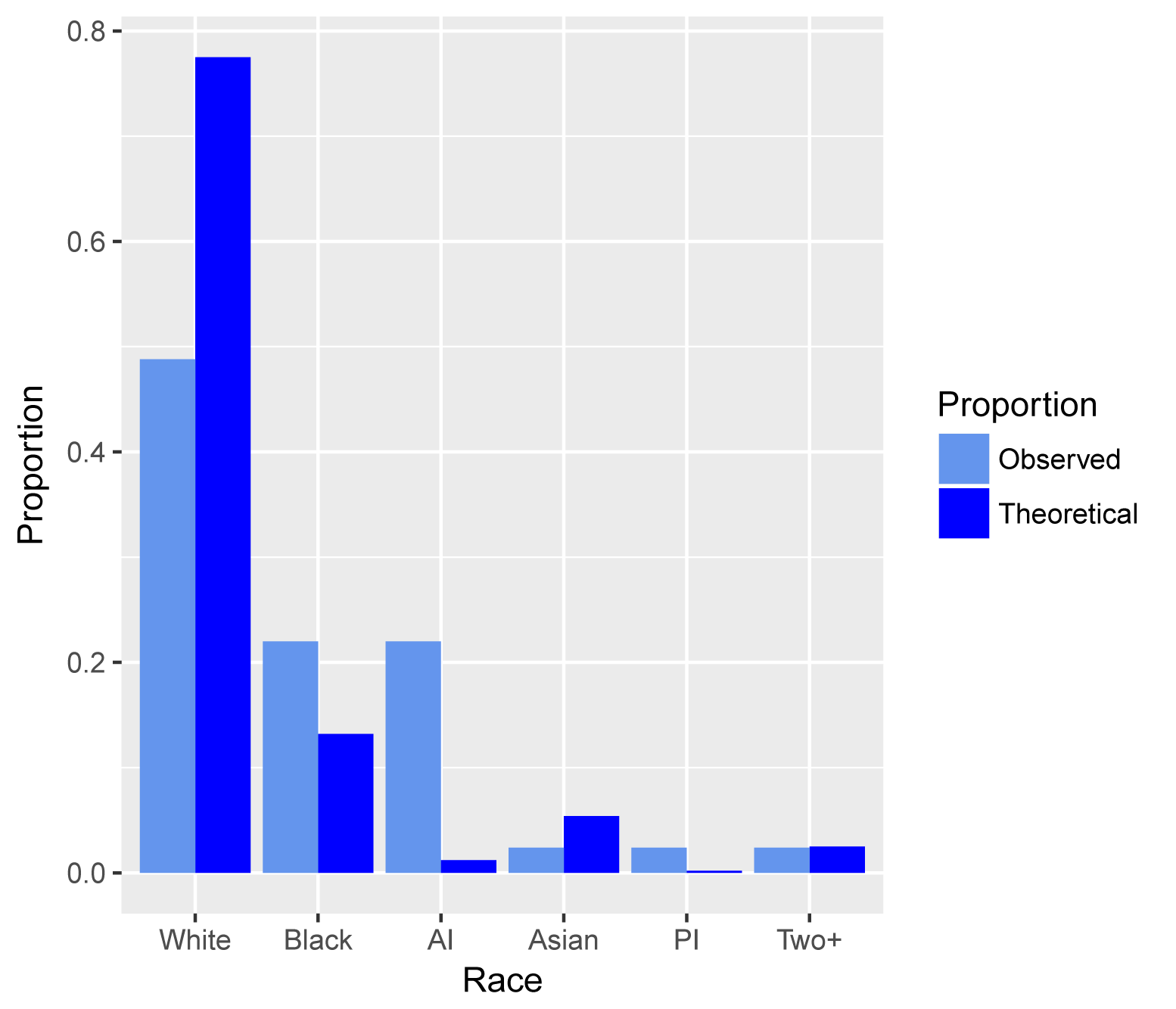
In order to facilitate plotting with R base graphics, the vector of counts is converted to proportions, and the theoretical and observed proportions are combined into a table, named XT.

 

See the Introduction to Tests for Nominal Variables chapter for a few additional options for how bar plots are plotted.

observed    = c(20, 9, 9, 1, 1, 1)
theoretical = c(0.775, 0.132, 0.012, 0.054, 0.002, 0.025)

Observed.prop    = observed / sum(observed)
Theoretical.prop = theoretical

Observed.prop    = round(Observed.prop, 3)
Theoretical.prop = round(Theoretical.prop, 3)

XT = rbind(Theoretical.prop, Observed.prop)

colnames(XT) = c("White", "Black", "AI", "Asian",  
                 "PI", "Two+")

XT

                 White Black    AI Asian    PI  Two+
Theoretical.prop 0.775 0.132 0.012 0.054 0.002 0.025
Observed.prop    0.488 0.220 0.220 0.024 0.024 0.024

barplot(XT,
        beside = T,
        xlab   = "Race",
        col    = c("cornflowerblue","blue"),
        legend = rownames(XT))

In order to plot with ggplot2, the table XT will be converted into a data frame in long format.

Race = c(colnames(XT), colnames(XT))

Race = factor(Race,
              levels=unique(colnames(XT)))

Proportion = c(rep("Theoretical", 6),
               rep("Observed", 6))

Value = c(XT[1,], XT[2,])

DF = data.frame(Race, Proportion, Value)

DF

    Race    Proportion Value
1  White   Theoretical 0.775
2  Black   Theoretical 0.132
3     AI   Theoretical 0.012
4  Asian   Theoretical 0.054
5     PI   Theoretical 0.002
6   Two+   Theoretical 0.025
7  White   Observed    0.488
8  Black   Observed    0.220
9     AI   Observed    0.220
10 Asian   Observed    0.024
11    PI   Observed    0.024
12  Two+   Observed    0.024

library(ggplot2)

ggplot(DF,
       aes(x = Race, y = Value, fill = Proportion)) +
       geom_bar(stat = 'identity', position = 'dodge') +
       scale_fill_manual(values = c("cornflowerblue", "blue")) +
       ylab("Proportion")

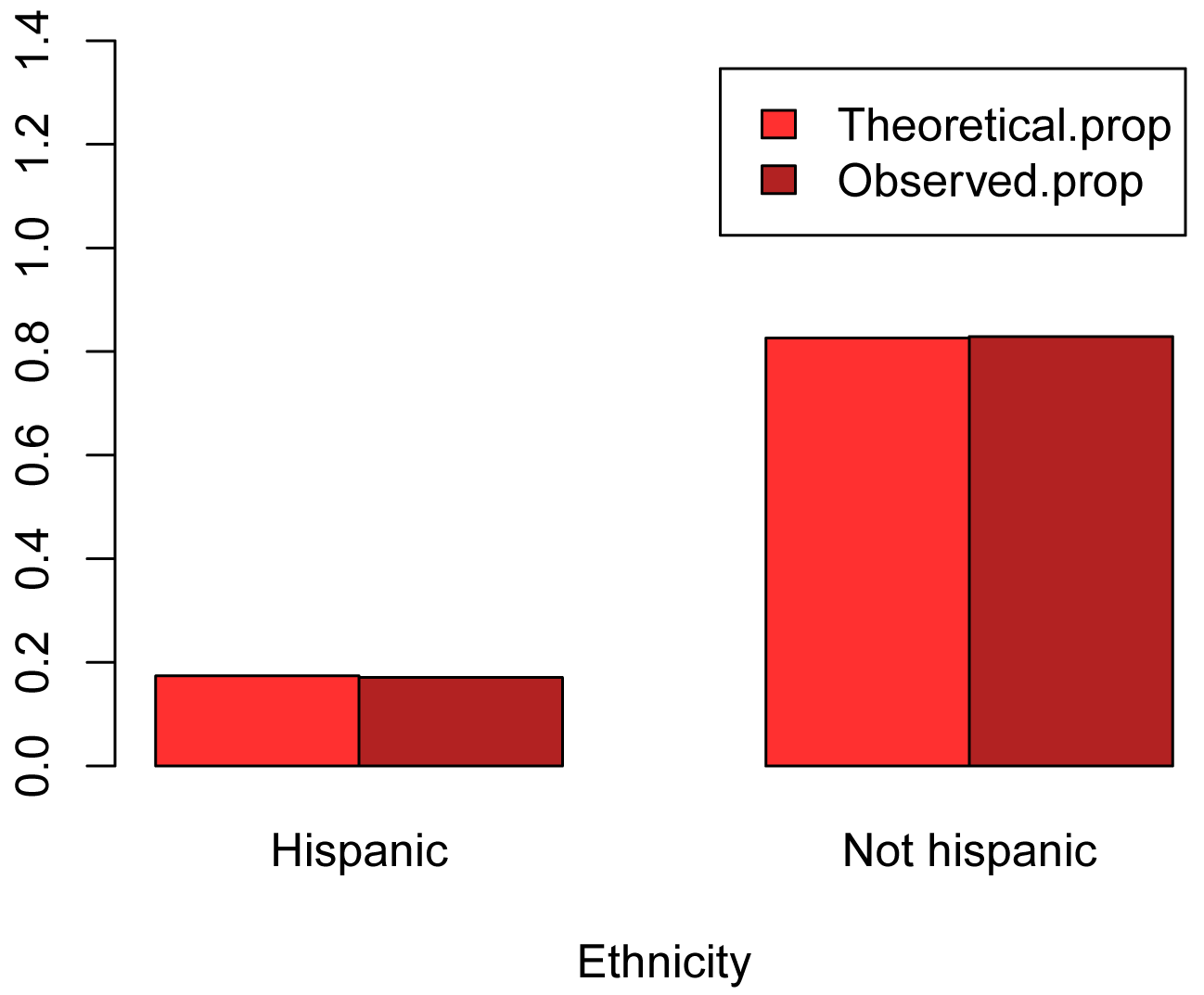
Ethnicity example

observed    = c(7, 34)
theoretical = c(0.174, 0.826)

Observed.prop    = observed / sum(observed)
Theoretical.prop = theoretical

Observed.prop    = round(Observed.prop, 3)
Theoretical.prop = round(Theoretical.prop, 3)

XT = rbind(Theoretical.prop, Observed.prop)

colnames(XT) = c("Hispanic", "Not Hispanic")

XT

                 Hispanic Not Hispanic
Theoretical.prop    0.174        0.826
Observed.prop       0.171        0.829

barplot(XT,
        beside = T,
        xlab   = "Ethnicity",
        col    = c("firebrick1","firebrick"),
        legend = rownames(XT),
        ylim   = c(0, 1.4))

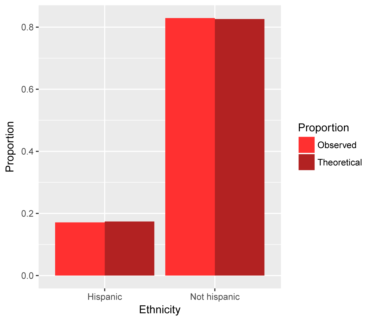
Ethnicity = c(colnames(XT), colnames(XT))

Ethnicity = factor(Ethnicity,
                   levels=unique(colnames(XT)))

Proportion = c(rep("Theoretical", 2), rep("Observed", 2))

Value = c(XT[1,], XT[2,])

DF = data.frame(Ethnicity, Proportion, Value)

DF

     Ethnicity    Proportion Value
1     Hispanic   Theoretical 0.174
2 Not Hispanic   Theoretical 0.826
3     Hispanic   Observed    0.171
4 Not Hispanic   Observed    0.829

library(ggplot2)

ggplot(DF,
       aes(x = Ethnicity, y = Value, fill = Proportion)) +
       geom_bar(stat = 'identity', position = 'dodge') +
       scale_fill_manual(values = c("firebrick1","firebrick")) +
       ylab("Proportion")

Optional: Multinomial test example with plot and confidence intervals

 

This is an example of a multinomial test that includes a bar plot showing confidence intervals.  The data is a simple vector of counts.

 

For a similar example using two-way count data which is organized into a data frame, see the "Examples of basic plots for nominal data" section in the Basic Plots chapter.

 

Walking to the store, Jerry Coyne observed the colors of nail polish on women’s toes (Coyne, 2016).  Presumably because that’s the kind of thing retired professors are apt to do.  He concluded that red was a more popular color but didn’t do any statistical analysis to support his conclusion.

Color of polish    Count
Red                19
None or clear       3
White               1
Green               1
Purple              2
Blue                2

We will use a multinomial goodness of fit test to determine if there is an overall difference in the proportion of colors (multinomial.test function in the EMT package).  The confidence intervals for each proportion can be found with the MultinomCI function in the DescTools package.  The data then need to be manipulated some so that we can plot the data as counts and not proportions.

 

Note here that the theoretical counts are simply 1 divided by the number of treatments.  In this case the null hypothesis is that the observed proportions are all the same.  In the examples above, the null hypothesis was that the observed proportions were not different than theoretical proportions.

 

The confidence intervals for each proportion can be used as a post-hoc test, to determine which proportions differ from each other, or to determine which proportions differ from 0.

nail.color  = c("Red", "None", "White", "Green", "Purple", "Blue")
observed    = c( 19,    3,      1,       1,       2,        2    )
theoretical = c( 1/6,   1/6,    1/6,     1/6,     1/6,      1/6  )


library(EMT)

multinomial.test(observed,
                 theoretical)

   ### This may take a while.  Use Monte Carlo for large numbers.

Exact Multinomial Test, distance measure: p

    Events    pObs    p.value
    237336       0          0

library(rcompanion)

cramerVFit(observed)

   ### Assumes equal proportions for theoretical values.

Cramer V

  0.6178

library(DescTools)

MCI = MultinomCI(observed,
                 conf.level=0.95,
                 method="sisonglaz")

MCI

            est    lwr.ci    upr.ci
[1,] 0.67857143 0.5357143 0.8423162
[2,] 0.10714286 0.0000000 0.2708876
[3,] 0.03571429 0.0000000 0.1994590
[4,] 0.03571429 0.0000000 0.1994590
[5,] 0.07142857 0.0000000 0.2351733
[6,] 0.07142857 0.0000000 0.2351733

### Order the levels, otherwise R will alphabetize them

Nail.color = factor(nail.color,
                    levels=unique(nail.color))


### For plot, Create variables of counts, and then wrap them into a data frame

Total = sum(observed)
Count = observed
Lower = MCI[,'lwr.ci'] * Total
Upper = MCI[,'upr.ci'] * Total

Data = data.frame(Nail.color, Count, Lower, Upper)

Data

  Count Lower     Upper
1    19    15 23.584853
2     3     0  7.584853
3     1     0  5.584853
4     1     0  5.584853
5     2     0  6.584853
6     2     0  6.584853

library(ggplot2)

ggplot(Data,                 ### The data frame to use.
       aes(x     = Nail.color,
           y     = Count)) +

    geom_bar(stat = "identity",
             color = "black",
             fill  = "gray50",
             width =  0.7) +

    geom_errorbar(aes(ymin  = Lower,
                      ymax  = Upper),
                      width = 0.2,
                      size  = 0.7,
                      color = "black"
                      ) +
    theme_bw() +
    theme(axis.title = element_text(face = "bold")) +

    ylab("Count of observations\n") +
    xlab("\nNail color")

Bar plot of the count of the color of women’s toenail polish observed by Jerry Coyne while walking to the store.  Error bars indicate 95% confidence intervals (Sison and Glaz method).

Optional readings

 

“Small numbers in chi-square and G–tests” in McDonald, J.H. 2014. Handbook of Biological Statistics. www.biostathandbook.com/small.html.

 

References

 

Cohen, J. 1988. Statistical Power Analysis for the Behavioral Sciences, 2nd Edition. Routledge.

 

Coyne, J. A. 2016. Why is red nail polish so popular? Why Evolution is True. whyevolutionistrue.com/2016/07/02/why-is-red-nail-polish-so-popular/.

 

“Chi-square Test of Goodness-of-Fit” in Mangiafico, S.S. 2015a. An R Companion for the Handbook of Biological Statistics, version 1.09. rcompanion.org/rcompanion/b_03.html.

 

“Exact Test of Goodness-of-Fit” in Mangiafico, S.S. 2015a. An R Companion for the Handbook of Biological Statistics, version 1.09. rcompanion.org/rcompanion/b_01.html.

 

“G–test of Goodness-of-Fit” in Mangiafico, S.S. 2015a. An R Companion for the Handbook of Biological Statistics, version 1.09. rcompanion.org/rcompanion/b_04.html.

 

“Repeated G–tests of Goodness-of-Fit” in Mangiafico, S.S. 2015a. An R Companion for the Handbook of Biological Statistics, version 1.09. rcompanion.org/rcompanion/b_09.html.

 

Exercises Beta

1. What do you conclude about whether the race of Alucard’s students match the proportions in the county?  Include, as appropriate:

•  The statistical test you are using, p-value from that test, conclusion of the test, and any other comments on the test.

 

•  The effect size and interpretation, or perhaps why you don’t want to rely on that information.

 

•  Description of the observed counts or proportions relative to the theoretical proportions.  Is there anything notable? 

 

•  Any other practical conclusions you wish to note.

 

2. What do you conclude about whether the ethnicity of Alucard’s students match the proportions in the county?  Include, as appropriate:

•  The statistical test you are using, p-value from that test, conclusion of the test, and any other comments on the test.

 

•  The effect size and interpretation, or perhaps why you don’t want to rely on that information.

 

•  Description of the observed counts or proportions relative to the theoretical proportions.  Is there anything notable? 

 

•  Any other practical conclusions you wish to note.

©2016 by Salvatore S. Mangiafico.
Rutgers Cooperative Extension, New Brunswick, NJ.

Non-commercial reproduction of this content, with attribution, is permitted.
For-profit reproduction without permission is prohibited.

If you use the code or information in this site in a published work, please cite it as a source.  Also, if you are an instructor and use this book in your course, please let me know.   My contact information is on the About the Author of this Book page.

Citation

Mangiafico, S.S. 2016. Summary and Analysis of Extension Program Evaluation in R, version 1.20.05, revised 2023. rcompanion.org/handbook/. (Pdf version: rcompanion.org/documents/RHandbookProgramEvaluation.pdf.)