Summary and Analysis of Extension Program Evaluation in R

Salvatore S. Mangiafico

Two-way Ordinal Regression with CLM

A two-way ordinal analysis of variance can address an experimental design with two independent variables, each of which is a factor variable.  The main effect of each independent variable can be tested, as well as the effect of the interaction of the two factors.

The example here looks at ratings for three instructors across four different questions.  The analysis will attempt to answer the questions:  a) Is there a significant difference in scores for different instructors?  b) Is there a significant difference in scores for different questions?  c) Is there a significant interaction effect of Instructor and Question?

Main effects and interaction effects are explained further in the Factorial ANOVA: Main Effects, Interaction Effects, and Interaction Plots chapter.

The clm function can specify more complex models with multiple independent variables of different types, but this book will not explore more complex examples.

Post-hoc analysis to determine which groups are different can be conducted on each significant main effect and on the interaction effect if it is significant.

Appropriate data

•  Two-way data

•  Dependent variable is ordered factor

•  Independent variables are factors with at least two levels or groups each

•  Observations between groups are not paired or repeated measures

Interpretation

A significant main effect can be interpreted as, “There was a significant difference among groups.”  Or, “There was a significant effect of Independent Variable.”

A significant interaction effect can be interpreted as, “There was a significant interaction effect between Independent Variable A and Independent Variable B.”

A significant post-hoc analysis indicates, “There was a significant difference between Group A and Group B”, and so on.

Packages used in this chapter

The packages used in this chapter include:

•  psych

•  FSA

•  lattice

•  ggplot2

•  ordinal

•  car

•  RVAideMemoire

•  rcompanion

•  multcomp

•  emmeans

The following commands will install these packages if they are not already installed:

if(!require(psych)){install.packages("psych")}
if(!require(FSA)){install.packages("FSA")}
if(!require(lattice)){install.packages("lattice")}
if(!require(ggplot2)){install.packages("ggplot2")}
if(!require(ordinal)){install.packages("ordinal")}
if(!require(car)){install.packages("car")}
if(!require(RVAideMemoire)){install.packages("RVAideMemoire")}
if(!require(rcompanion)){install.packages("rcompanion")}
if(!require(multcomp)){install.packages("multcomp")}
if(!require(emmeans)){install.packages("emmeans")}

Two-way ordinal regression example

Data = read.table(header=TRUE, stringsAsFactors=TRUE, text="

Instructor  Question       Likert
 Fuu         Informative     8
 Fuu         Informative     9
 Fuu         Informative     9
 Fuu         Informative     8
 Fuu         Delivery       10
 Fuu         Delivery        9
 Fuu         Delivery        8
 Fuu         Delivery        8
 Fuu         VisualAides     7
 Fuu         VisualAides     7
 Fuu         VisualAides     6
 Fuu         VisualAides     7
 Fuu         AnswerQuest     8
 Fuu         AnswerQuest     9
 Fuu         AnswerQuest     9
 Fuu         AnswerQuest     8
 Jin         Informative     7
 Jin         Informative     8
 Jin         Informative     6
 Jin         Informative     5
 Jin         Delivery        8
 Jin         Delivery        8
 Jin         Delivery        9
 Jin         Delivery        6
 Jin         VisualAides     5
 Jin         VisualAides     6
 Jin         VisualAides     7
 Jin         VisualAides     7
 Jin         AnswerQuest     8
 Jin         AnswerQuest     7
 Jin         AnswerQuest     6
 Jin         AnswerQuest     6
 Mugen       Informative     5
 Mugen       Informative     4
 Mugen       Informative     3
 Mugen       Informative     4
 Mugen       Delivery        8
 Mugen       Delivery        9
 Mugen       Delivery        8
 Mugen       Delivery        7
 Mugen       VisualAides     5
 Mugen       VisualAides     4
 Mugen       VisualAides     4
 Mugen       VisualAides     5
 Mugen       AnswerQuest     6
 Mugen       AnswerQuest     7
 Mugen       AnswerQuest     6
 Mugen       AnswerQuest     7
")


### Order levels of the factor; otherwise R will alphabetize them

Data$Instructor = factor(Data$Instructor,
                      levels=unique(Data$Instructor))
                                    


### Create a new variable which is the likert scores as an ordered factor

Data$Likert.f = factor(Data$Likert,
                       ordered = TRUE)


###  Check the data frame

library(psych)

headTail(Data)

str(Data)

summary(Data)

Summarize data treating Likert scores as factors

xtabs( ~ Instructor + Likert.f,
      data = Data)

          Likert.f
Instructor 3 4 5 6 7 8 9 10
     Fuu   0 0 0 1 3 6 5  1
     Jin   0 0 2 5 4 4 1  0
     Mugen 1 4 3 2 3 2 1  0

xtabs( ~ Question + Likert.f,
      data = Data)

          
             Likert.f
Question      3 4 5 6 7 8 9 10
  AnswerQuest 0 0 0 4 3 3 2  0
  Delivery    0 0 0 1 1 6 3  1
  Informative 1 2 2 1 1 3 2  0
  VisualAides 0 2 3 2 5 0 0  0

xtabs( ~ Instructor + Likert.f + Question,
      data = Data)

, , Question = AnswerQuest

          Likert.f
Instructor 3 4 5 6 7 8 9 10
     Fuu   0 0 0 0 0 2 2  0
     Jin   0 0 0 2 1 1 0  0
     Mugen 0 0 0 2 2 0 0  0

, , Question = Delivery

          Likert.f
Instructor 3 4 5 6 7 8 9 10
     Fuu   0 0 0 0 0 2 1  1
     Jin   0 0 0 1 0 2 1  0
     Mugen 0 0 0 0 1 2 1  0

, , Question = Informative

          Likert.f
Instructor 3 4 5 6 7 8 9 10
     Fuu   0 0 0 0 0 2 2  0
     Jin   0 0 1 1 1 1 0  0
     Mugen 1 2 1 0 0 0 0  0

, , Question = VisualAides

          Likert.f
Instructor 3 4 5 6 7 8 9 10
     Fuu   0 0 0 1 3 0 0  0
     Jin   0 0 1 1 2 0 0  0
     Mugen 0 2 2 0 0 0 0  0

Bar plots by group

library(lattice)

histogram(~ Likert.f | Instructor,
          data=Data,
          layout=c(1,3)      #  columns and rows of individual plots
          )

library(lattice)

histogram(~ Likert.f | Question,
          data=Data,
          layout=c(1,4)      #  columns and rows of individual plots
          )

library(lattice)

histogram(~ Likert.f | Instructor + Question,
          data=Data,
          layout=c(3,4)      #  columns and rows of individual plots
          )

Summarize data treating Likert scores as numeric

library(FSA)

Summarize(Likert ~ Instructor,
          data=Data,
          digits=3)

  Instructor  n  mean    sd min   Q1 median Q3 max percZero
1        Fuu 16 8.125 1.025   6 7.75    8.0  9  10        0
2        Jin 16 6.812 1.167   5 6.00    7.0  8   9        0
3      Mugen 16 5.750 1.770   3 4.00    5.5  7   9        0

library(FSA)

Summarize(Likert ~ Question,
          data=Data,
          digits=3)

     Question  n  mean    sd min   Q1 median Q3 max percZero
1 AnswerQuest 12 7.250 1.138   6 6.00    7.0  8   9        0
2    Delivery 12 8.167 1.030   6 8.00    8.0  9  10        0
3 Informative 12 6.333 2.103   3 4.75    6.5  8   9        0
4 VisualAides 12 5.833 1.193   4 5.00    6.0  7   7        0

library(FSA)

Summarize(Likert ~ Instructor + Question,
          data=Data,
          digits=3)

   Instructor    Question n mean    sd min   Q1 median   Q3 max percZero
1         Fuu AnswerQuest 4 8.50 0.577   8 8.00    8.5 9.00   9        0
2         Jin AnswerQuest 4 6.75 0.957   6 6.00    6.5 7.25   8        0
3       Mugen AnswerQuest 4 6.50 0.577   6 6.00    6.5 7.00   7        0
4         Fuu    Delivery 4 8.75 0.957   8 8.00    8.5 9.25  10        0
5         Jin    Delivery 4 7.75 1.258   6 7.50    8.0 8.25   9        0
6       Mugen    Delivery 4 8.00 0.816   7 7.75    8.0 8.25   9        0
7         Fuu Informative 4 8.50 0.577   8 8.00    8.5 9.00   9        0
8         Jin Informative 4 6.50 1.291   5 5.75    6.5 7.25   8        0
9       Mugen Informative 4 4.00 0.816   3 3.75    4.0 4.25   5        0
10        Fuu VisualAides 4 6.75 0.500   6 6.75    7.0 7.00   7        0
11        Jin VisualAides 4 6.25 0.957   5 5.75    6.5 7.00   7        0
12      Mugen VisualAides 4 4.50 0.577   4 4.00    4.5 5.00   5        0

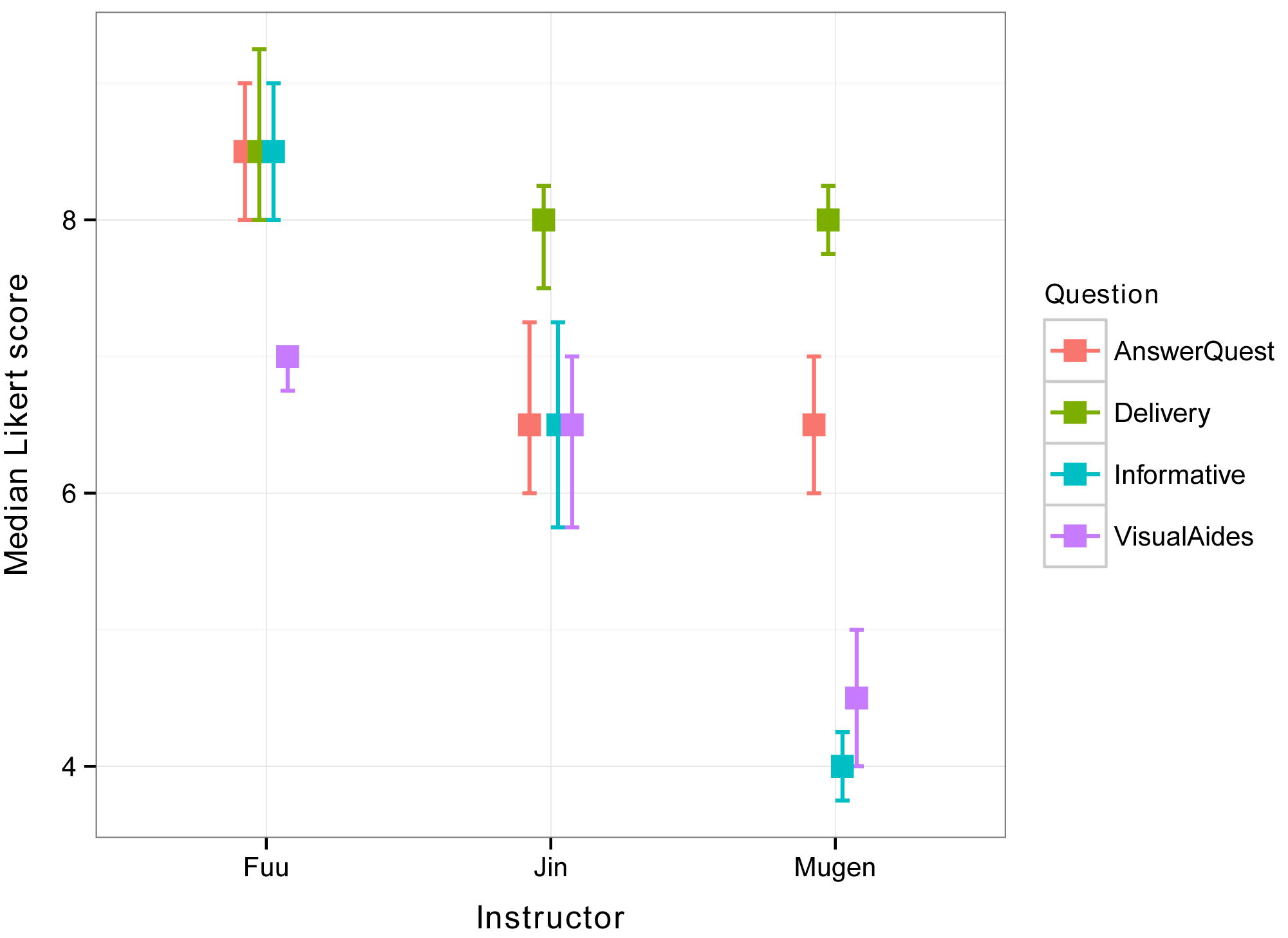
Produce interaction plot with medians and quantiles

The following plot shows medians for the interaction of Instructor and Question, with error bars showing the 1^st quartile and 3^rd quartile for each median.

library(FSA)

Sum = Summarize(Likert ~ Instructor + Question,
                data=Data,
                digits=3)

Sum


library(ggplot2)

pd = position_dodge(.2)

ggplot(Sum, aes(x=Instructor,
                y=median,
                color=Question)) +
    geom_errorbar(aes(ymin=Q1,
                      ymax=Q3),
                   width=.2, size=0.7, position=pd) +
    geom_point(shape=15, size=4, position=pd) +
    theme_bw() +
    theme(axis.title = element_text(face = "bold"))+

    ylab("Median Likert score")

Two-way ordinal regression

In the model notation in the clm function, here, Likert.f is the dependent variable and Instructor and Question are the independent variables.  The term Instructor:Question adds the interaction effect of these two independent variables to the model.  The data= option indicates the data frame that contains the variables.  For the meaning of other options, see ?clm.

Here the threshold = "symmetric" option is used in order to avoid errors.  This option does not need to be used routinely.

Define model and analyses of deviance

library(ordinal)

model = clm(Likert.f ~ Instructor + Question + Instructor:Question,
            data = Data,
            threshold="symmetric")

Analysis of deviance

anova(model, type="II")

Type II Analysis of Deviance Table with Wald chi-square tests

                    Df  Chisq Pr(>Chisq)   
Instructor           2 26.748  1.555e-06 ***
Question             3 24.596  1.876e-05 ***
Instructor:Question  6 18.194   0.005766 **

Alternate analysis of deviance analysis

library(car)

library(RVAideMemoire)

Anova.clm(model, type = "II")

Analysis of Deviance Table (Type II tests)

                    LR Chisq Df Pr(>Chisq)   
Instructor            32.157  2  1.040e-07 ***
Question              28.248  3  3.221e-06 ***
Instructor:Question   24.326  6  0.0004548 ***

p-value for model and pseudo R-squared

The p-value for the model and a pseudo R-squared value can be determined with the nagelkerke function.  It is not clear to me which pseudo R-squared value would be most appropriate for an ordinal regression model.

library(rcompanion)

nagelkerke(model)

$Pseudo.R.squared.for.model.vs.null

                             Pseudo.R.squared
McFadden                             0.400602
Cox and Snell (ML)                   0.775956
Nagelkerke (Cragg and Uhler)         0.794950


$Likelihood.ratio.test

 Df.diff LogLik.diff  Chisq    p.value
     -11     -35.902 71.804 5.5398e-11

Post-hoc tests

For clm model objects, the emmean, SE, LCL, and UCL values should be ignored, unless specific options in emmeans are selected.

Because the interaction term in the model was significant, the group separation for the interaction effect is explored.

library(emmeans)

marginal = emmeans(model,
                   ~ Instructor + Question)

pairs(marginal,
      adjust="tukey")

library(multcomp)

cld(marginal, Letters=letters)

Instructor Question    emmean    SE  df asymp.LCL asymp.UCL .group
 Mugen      Informative -6.663 1.419 Inf    -9.444     -3.88  a   
 Mugen      VisualAides -5.263 1.279 Inf    -7.770     -2.76  ab  
 Jin        VisualAides -0.435 0.944 Inf    -2.284      1.41   bc 
 Jin        Informative  0.000 1.055 Inf    -2.067      2.07   bcd
 Mugen      AnswerQuest  0.000 0.848 Inf    -1.663      1.66    c 
 Jin        AnswerQuest  0.435 0.944 Inf    -1.415      2.28    cde
 Fuu        VisualAides  0.553 0.846 Inf    -1.107      2.21    cd
 Jin        Delivery     3.490 1.319 Inf     0.904      6.08    cde
 Mugen      Delivery     3.713 1.225 Inf     1.311      6.11    cde
 Fuu        AnswerQuest  5.263 1.279 Inf     2.756      7.77     de
 Fuu        Informative  5.263 1.279 Inf     2.756      7.77     de
 Fuu        Delivery     5.783 1.378 Inf     3.082      8.48      e

Confidence level used: 0.95
P value adjustment: tukey method for comparing a family of 12 estimates
significance level used: alpha = 0.05

NOTE: Compact letter displays can be misleading
      because they show NON-findings rather than findings.
      Consider using 'pairs()', 'pwpp()', or 'pwpm()' instead.


   ### Groups sharing a letter in .group are not significantly different

   ### Remember to ignore “emmean”, “SE”, “LCL”, and “UCL” with CLM

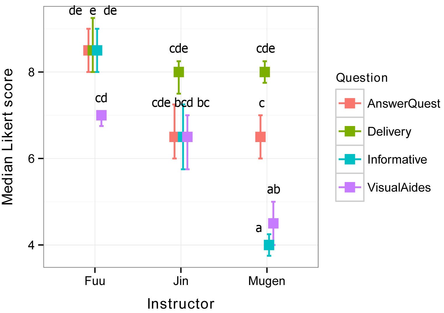
Interaction plot with group separation letters

Group separation letters can be added manually to an interaction plot.

Groups sharing a letter are not significantly different.  In this case, because so many groups share a letter, it is difficult to interpret this plot.  One approach would be to look at differences among instructors for each question.  Looking at AnswerQuest, Fuu’s scores are not statistically different than Jin’s (because they share the letters d and e), but Fuu’s scores are different than Mugen’s (because they share no letters).  So, we can conclude for this question, that Fuu’s scores are significantly greater than Mugen’s.  And so on.
 

Check model assumptions

nominal_test(model)

Tests of nominal effects

formula: Likert.f ~ Instructor + Question + Instructor:Question
                    Df  logLik    AIC    LRT Pr(>Chi)
<none>                 -53.718 137.44               
Instructor           6 -49.812 141.62 7.8121   0.2522
Question             9 -50.182 148.37 7.0711   0.6297
Instructor:Question 

   ###  No violation in assumptions.

scale_test(model)

Tests of scale effects

formula: Likert.f ~ Instructor + Question + Instructor:Question
                    Df  logLik    AIC    LRT Pr(>Chi) 
<none>                 -53.718 137.44                 
Instructor           2 -51.669 137.34 4.0985  0.12883 
Question             3 -50.534 137.07 6.3669  0.09506 .
Instructor:Question                                   

Warning message:
(-1) Model failed to converge with max|grad| = 1.70325e-06 (tol = 1e-06)
In addition: maximum number of consecutive Newton modifications reached

   ###  This test failed, but the results suggest no violation of assumptions.

©2016 by Salvatore S. Mangiafico.
Rutgers Cooperative Extension, New Brunswick, NJ.

Non-commercial reproduction of this content, with attribution, is permitted.
For-profit reproduction without permission is prohibited.

If you use the code or information in this site in a published work, please cite it as a source.  Also, if you are an instructor and use this book in your course, please let me know.   My contact information is on the About the Author of this Book page.

Citation

Mangiafico, S.S. 2016. Summary and Analysis of Extension Program Evaluation in R, version 1.20.05, revised 2023. rcompanion.org/handbook/. (Pdf version: rcompanion.org/documents/RHandbookProgramEvaluation.pdf.)